Ocean Wave Energy Flux Forecasting: A Stacking Ensemble (Part 2)
Published:
Series: Wave Energy Part: 3 (Flux Forecasting: Stacking Ensemble)
Introduction
“Multi-ridge regression,” or stacking with a ridge regression meta-model, means using L2-regularized linear regression to combine the predictions of several base machine learning models. In this part, the base models are Ridge Regression, Random Forest, and LightGBM. For background on the individual techniques, see the Machine Learning section of this site.
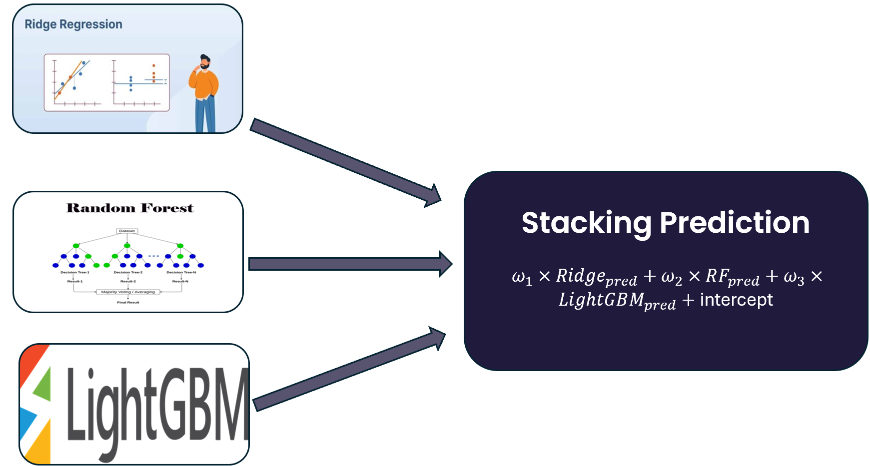
How ridge regression combines the base models:
- Stacking meta-regressor. Instead of simple averaging, a ridge regression model treats the predictions of the individual base models as input features to predict the final target.1234
- L2 penalty control. The ridge penalty stops the meta-model from assigning overly large or unstable weights to any single base model, and handles correlated base-model predictions gracefully.563
- Bias-variance balance. It shrinks the coefficients of weak or redundant base models toward zero, which improves generalization on unseen data.
Data, walk-forward folds, and the best-lag choices per (target, lead time) are all reused unchanged from Part 1; only the modeling stage changes here. For each target and lead time, RFE feature selection is re-run (since the best feature set can differ across model types), and the three base models are each fit and validated before the ridge meta-model learns how to combine them.
Results
2.1 Base Models vs. Stacking Ensemble
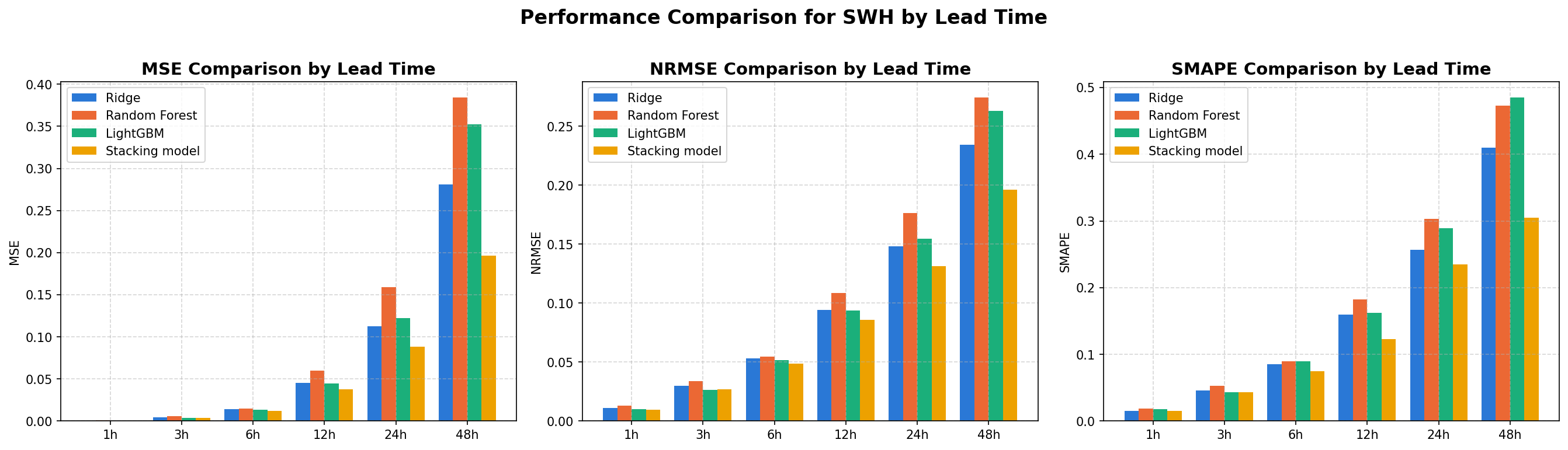
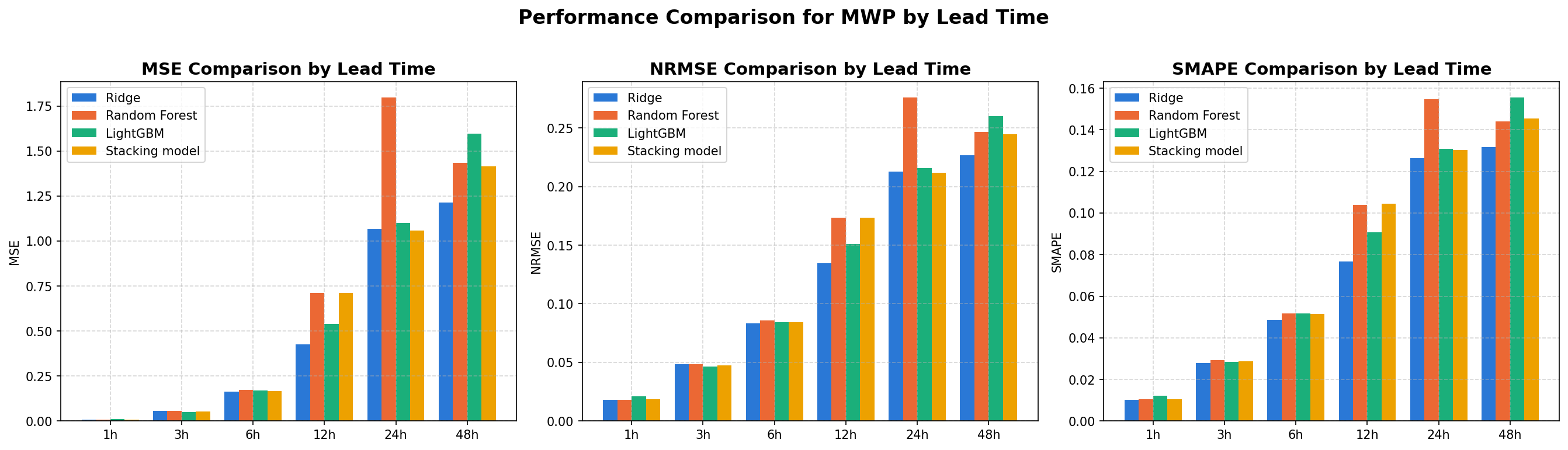
Comparing MSE, NRMSE, and SMAPE across all four models (the three base models plus the stacking ensemble) by lead time:
The stacked model’s own test-set metrics, together with the ridge meta-model’s learned weight on each base model:
Significant wave height (Hs / swh):
| Lead (h) | MAE | RMSE | NRMSE | SMAPE | R² | ridge_coef | rf_coef | lgbm_coef |
|---|---|---|---|---|---|---|---|---|
| 1 | 0.02 | 0.02 | 0.01 | 0.02 | 1.00 | 0.29 | 0.35 | 0.36 |
| 3 | 0.04 | 0.06 | 0.03 | 0.04 | 0.99 | 0.09 | 0.32 | 0.59 |
| 6 | 0.08 | 0.11 | 0.05 | 0.07 | 0.96 | 0.12 | 0.32 | 0.57 |
| 12 | 0.13 | 0.19 | 0.09 | 0.12 | 0.86 | -0.09 | 0.08 | 1.08 |
| 24 | 0.23 | 0.30 | 0.13 | 0.24 | 0.69 | 0.17 | -0.71 | 1.87 |
| 48 | 0.34 | 0.44 | 0.20 | 0.30 | 0.33 | 1.40 | 0.08 | 0.45 |
Mean wave period (Te / mwp):
| Lead (h) | MAE | RMSE | NRMSE | SMAPE | R² | ridge_coef | rf_coef | lgbm_coef |
|---|---|---|---|---|---|---|---|---|
| 1 | 0.07 | 0.09 | 0.02 | 0.01 | 0.99 | 0.24 | 0.25 | 0.51 |
| 3 | 0.18 | 0.23 | 0.05 | 0.03 | 0.94 | 0.02 | 0.34 | 0.63 |
| 6 | 0.32 | 0.41 | 0.08 | 0.05 | 0.82 | 0.03 | 0.46 | 0.49 |
| 12 | 0.66 | 0.84 | 0.17 | 0.10 | 0.23 | -0.55 | 0.08 | 1.47 |
| 24 | 0.84 | 1.03 | 0.21 | 0.13 | -0.13 | -0.01 | -0.08 | 1.20 |
| 48 | 0.95 | 1.19 | 0.24 | 0.15 | -0.49 | 1.14 | -2.24 | 9.63* |
*The mwp/48h lgbm_coef is reported as 9.63 in the raw results; given the intercept for that row is also unusually large in magnitude, this row’s meta-model fit is clearly unstable rather than a meaningful weighting (see Simplifications below).
Comparing these to Part 1’s pure-LightGBM test R² at the same leads is the real payoff of the stacking approach: for Hs, stacking is better everywhere from 12h onward, and 48h flips from clearly negative (-0.66 in Part 1) to a solidly positive 0.33 here. For Te, the picture is mixed rather than uniformly better: stacking is roughly even with pure LightGBM through 6h, but actually a bit worse at 12h and 24h, and only marginally less negative at 48h. So the ensemble recovers real long-lead skill for wave height specifically, not for wave period.
The meta-model’s coefficients also confirm the ridge penalty is doing real work: the weight on each base model shifts noticeably by lead time rather than settling on one fixed blend, and it occasionally goes negative (e.g. rf_coef at swh/24h and mwp/48h), where the meta-model is actively subtracting a correlated base prediction rather than simply averaging it in.
2.2 Time Series Forecasting
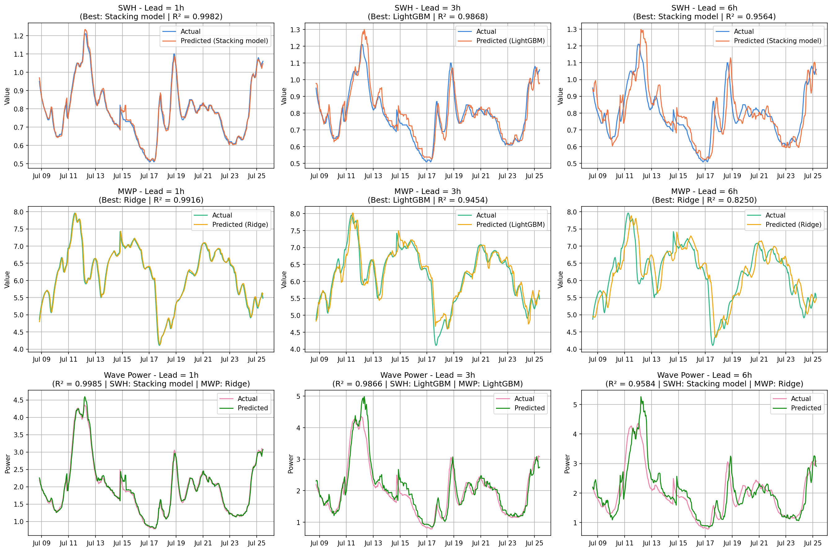
Each base model tends to lead at a different point in the lead-time range, with Random Forest not winning outright at any of them. At the shorter leads (1h, 3h, 6h), the stacking model, LightGBM, and Ridge each take turns being the best performer depending on lead time. At the longer leads (12h through 48h), the stacking model has the best overall performance for wave height, but for wave period stacking only wins at 24h; Ridge Regression wins on its own at 12h and 48h.

Simplifications
- The meta-model is fit on validation-set predictions only (
meta_X_valid), a fairly small sample to learn three coefficients and an intercept from; the unstable mwp/48h row above is a direct symptom of this. - “Best model per lead” is chosen by test-set RMSE, which is a look at the test set itself rather than a fully blind selection; treat the Section 2.2 comparisons as descriptive of this run, not as a guaranteed ranking on unseen data.
- Only one of six walk-forward folds is shown, the same limitation carried over from Part 1.
- Wave power is still a derived, ex-post quantity: each target’s best model is picked independently, then combined multiplicatively, so Hs and Te errors compound in the power estimate exactly as in Part 1.
Conclusion
Stacking Ridge Regression, Random Forest, and LightGBM with a ridge meta-model answers the question Part 1 ended on: it does recover meaningful long-lead skill, but only for significant wave height, where 48h R² turns from negative to a positive 0.33. Mean wave period doesn’t get the same benefit: stacking is roughly a wash or slightly worse than plain LightGBM at 12-24h. Part 3 moves to probabilistic forecasting (Quantile Regression, Quantile Regression Forest, and bootstrapped residuals), which should matter most exactly where these first two parts have shown point forecasts breaking down.
References
Code
- Stacking_Ensemble_ERA5.py: loads Part 1’s data and best-lag table, fits the three base models and the ridge meta-model per (target, lead), and produces all figures above.
- plot_all.py: plotting helpers shared across figures.
- stacking_ensemble_results.csv: the full results table above, including the meta-model coefficients.
Next: Part 3 turns to probabilistic forecasting (Quantile Regression, Quantile Regression Forest, and bootstrapped residuals) to put uncertainty bounds around the point forecasts from Parts 1 and 2.
“Bagging vs Boosting vs Stacking in Machine Learning”, GrabNGoInfo. ↩
“Building Multi-Output Regression Models: Linear & Ridge Regression”, LinkedIn. ↩
“Understanding Ridge Regression”, Certometer. ↩ ↩2
“Stacking ensemble machine learning”, ScienceDirect. ↩
“What is Ridge Regression?”, GeeksforGeeks. ↩