Ocean Wave Energy Flux Forecasting using LightGBM (Part 1)
Published:
Series: Wave Energy Part: 2 (Flux Forecasting — LightGBM)
Part 1 of this series introduced wave energy conversion and the physics behind ocean waves. This post starts the forecasting side of the series.
Introduction
Wave energy flux also called wave power per unit crest length is the rate at which energy is transmitted by ocean waves across a unit width of wave front. It represents how much energy flows through the sea surface due to wave motion.
The deep-water wave energy flux is:
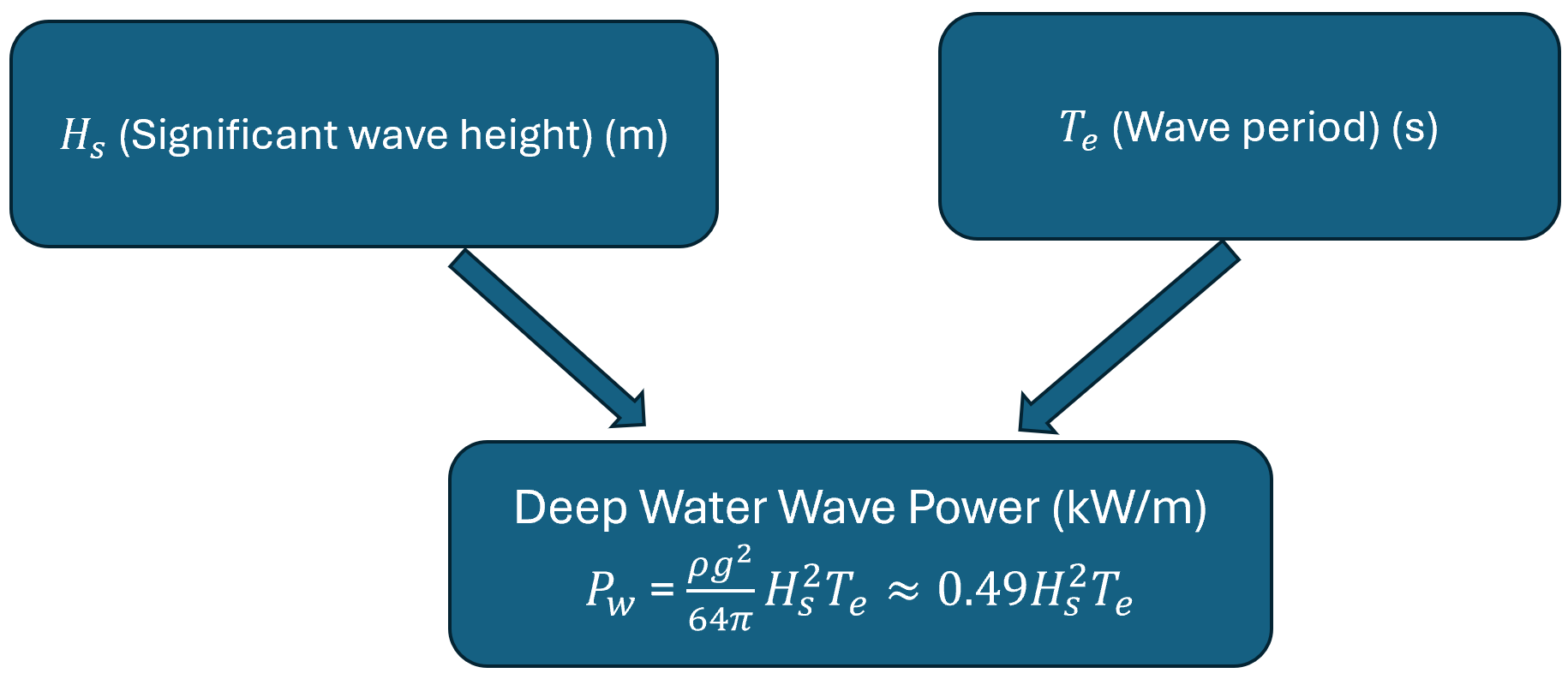
\[P=\frac{\rho g^2}{64\pi}H_s^2 T_e\]or, in simplified engineering form:
\[P \approx 0.49\, H_s^2 T_e \quad \text{[kW/m]}\]Where:
- ρ = water density (≈ 1025 kg/m³)
- g = gravitational acceleration (9.81 m/s²)
- Hs = significant wave height (m)
- Te = peak wave period (s)
Accurate short-term prediction of wave power flux is essential for real-time energy control, resource assessment, and operational decision-making in wave energy systems. Reliable forecasts directly support the efficiency, safety, and economic performance of wave energy converters operating in highly variable marine conditions.
Models for predicting wave power flux can be categorized into two types:
- Physical models
- Machine learning models
Physical models simulate the generation, propagation, transformation, and dissipation of ocean waves by solving the spectral action balance equation. This equation incorporates wind forcing, nonlinear wave interactions, and energy dissipation mechanisms. The most widely used third-generation physical models include the Wave Model (WAM), WAVEWATCH III (WW3), the European Centre for Medium-Range Weather Forecasts (ECMWF) model, and Simulating Waves Nearshore (SWAN). However, physics-based models involve high computational cost and complex processes, and are generally used for wide-area, medium-to-long-term marine weather forecasting; they can struggle with short-term, highly nonlinear variations in wave power flux. They also rely heavily on accurate meteorological input and complex parameterization, which makes them less adaptable and less efficient for real-time, site-specific forecasting, especially in rapidly changing or data-sparse environments.1
In this context, advances in artificial intelligence have driven growing interest in data-driven approaches to wave power flux prediction, particularly through machine learning models. This series builds up wave energy flux forecasting in three stages: an autoregressive LightGBM model in this post (Part 1); a multi-model stacking ensemble (Ridge Regression, Random Forest, and LightGBM) in Part 2; and probabilistic forecasting (Quantile Regression, Quantile Regression Forest, and bootstrapped residuals) in Part 3.
Methodology
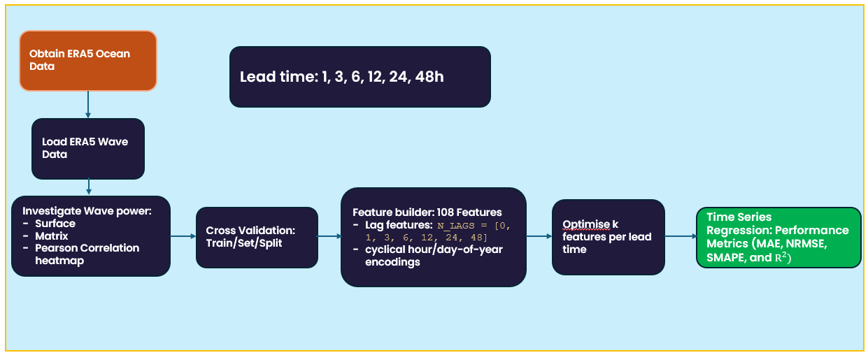
We obtain ERA5 ocean data from the ECMWF Climate Data Store: ERA5 hourly data on single levels from 1940 to present.
Data range: 2024-01-01 00:00 UTC to 2026-07-25. The lead time for short-term forecasting spans 1 to 48 hours. We first look at the theoretical wave power surface, the power matrix, and a Pearson correlation heatmap, then build lag features and cyclical hour/day-of-year encodings.
To choose the number of features (k) to keep per lead time, we use recursive feature elimination:
- Start with all features, fit LightGBM, score on the validation set.
- Drop the 5 weakest by importance, repeat down to 1 feature.
- Pick the feature count with the best validation R².
- Run this separately per target and per lead time — each combination gets its own k.
The resulting model is then evaluated on the held-out test set with several regression metrics: MAE, RMSE, NRMSE, SMAPE, and R².
2.1 Data Acquisition
Data acquisition goes through the ERA5 CDS API (an API key from the Climate Data Store is required). The site is Aguçadoura, near the Port of Viana do Castelo in northern Portugal — the same stretch of coast best known for the Aguçadoura Wave Farm, which briefly ran the world’s first commercial wave energy converters (Pelamis) in 2008.
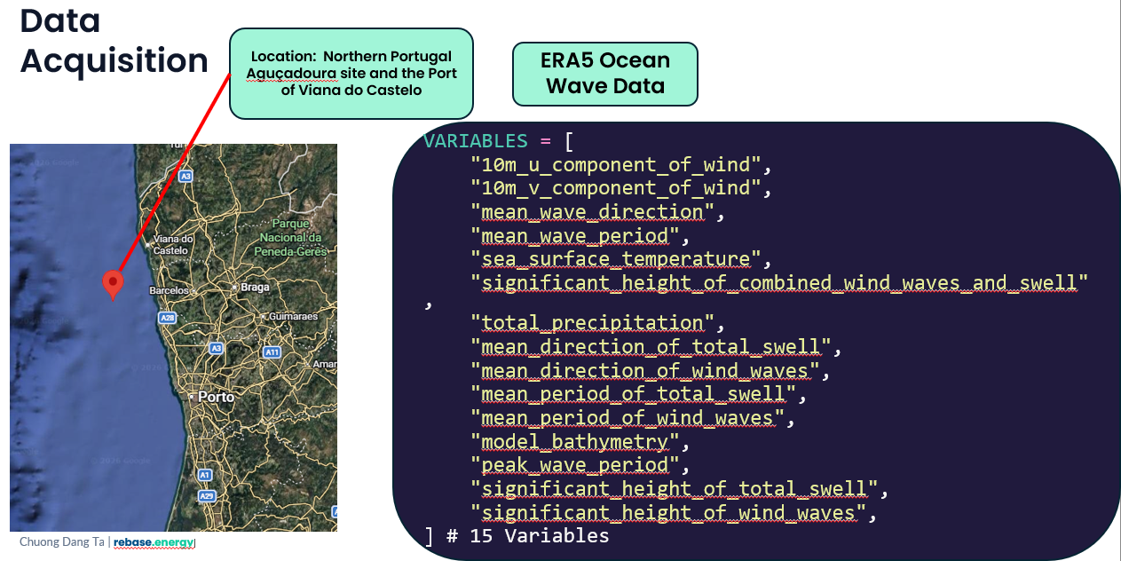
ERA5 wave and meteorological variables:
| Variable | Meaning |
|---|---|
| valid_time | Timestamp of the data in UTC; when the model output is valid. |
| latitude | Latitude of the grid point (north–south position). |
| longitude | Longitude of the grid point (east–west position). |
| u10 | 10-m east–west wind component; positive values mean wind blowing eastward. |
| v10 | 10-m north–south wind component; positive values mean wind blowing northward. |
| sst | Sea surface temperature; temperature of the ocean skin layer. |
| number | Ensemble member index (0–9); identifies which ensemble forecast is used. |
| expver | Experiment version; internal ECMWF metadata for dataset versioning. |
| tp | Total precipitation (m); accumulated rainfall and snowfall converted to water. |
| mwd | Mean wave direction; average direction of all waves in the spectrum. |
| mwp | Mean wave period; energy period used for wave power calculations. |
| swh | Significant wave height; average height of the highest one-third of waves. |
| mdts | Mean direction of total swell; direction of long-period swell waves. |
| mdww | Mean direction of wind waves; direction of locally generated wind waves. |
| mpts | Mean period of total swell; average period of swell waves. |
| mpww | Mean period of wind waves; average period of wind-generated waves. |
| wmb | Wave mean bandwidth; spectral width indicating how broad the wave spectrum is. |
| pp1d | Peak period (first spectral moment); dominant wave period. |
| shts | Significant height of total swell; height of long-period swell waves. |
| shww | Significant height of wind waves; height of short-period wind waves. |
The two forecast targets are Hs and Te, corresponding to swh and mwp in the dataset respectively.
2.2 Data Investigation
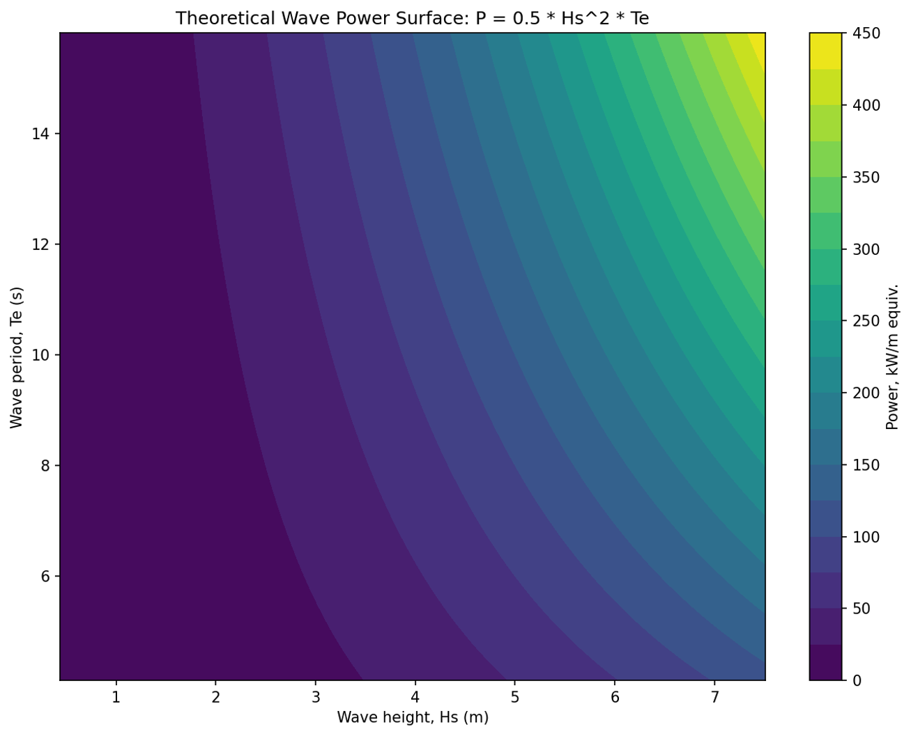
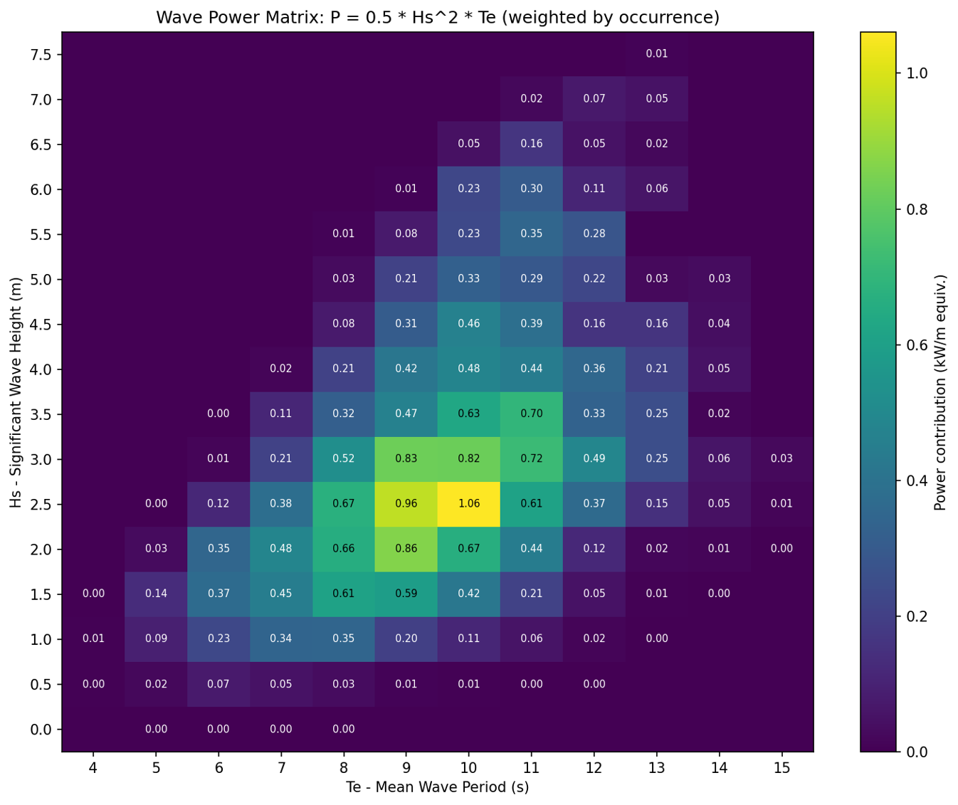
The theoretical wave power surface, P = 0.5 Hs² Te, is plotted directly over the observed range of Hs and Te (using the rounded coefficient 0.5 here rather than the more precise 0.49 physical constant — a common simplification for a diagnostic surface, since Hs and Te are the actual forecast targets and power itself is only computed downstream as a derived quantity, not something the model is trained on directly).
Weighting that same surface by how often each (Hs, Te) combination actually occurs in the data gives the power matrix below. Most of the wave power at this site comes from the range Te = 8–10 s and Hs = 2.0–3.0 m — this is the combination that matters most for resource assessment, since a rarer sea state with higher theoretical power can still contribute less energy overall than a common, moderate one.
2.3 Pearson Correlation and Walk-Forward Cross-Validation
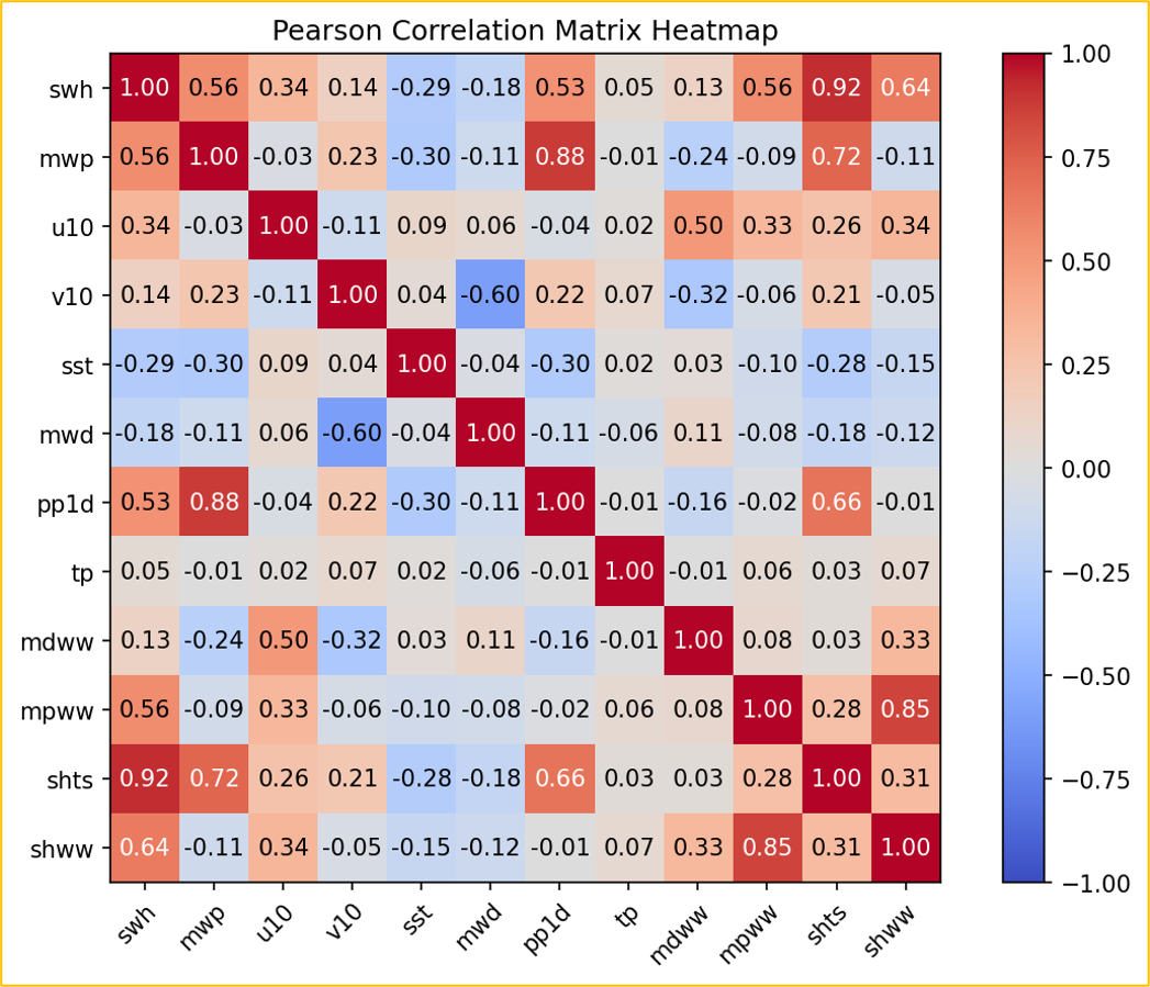
Before building lag features, a Pearson correlation heatmap gives a quick, interpretable screen of which variables are linearly related to the targets:
\[r_{xy} = \frac{\sum_i (x_i-\bar{x})(y_i-\bar{y})}{\sqrt{\sum_i (x_i-\bar{x})^2}\sqrt{\sum_i (y_i-\bar{y})^2}}\]tp (total precipitation) was dropped after this step — it showed essentially no linear correlation with either target, which is physically sensible, since instantaneous rainfall isn’t itself a wave-generating variable.
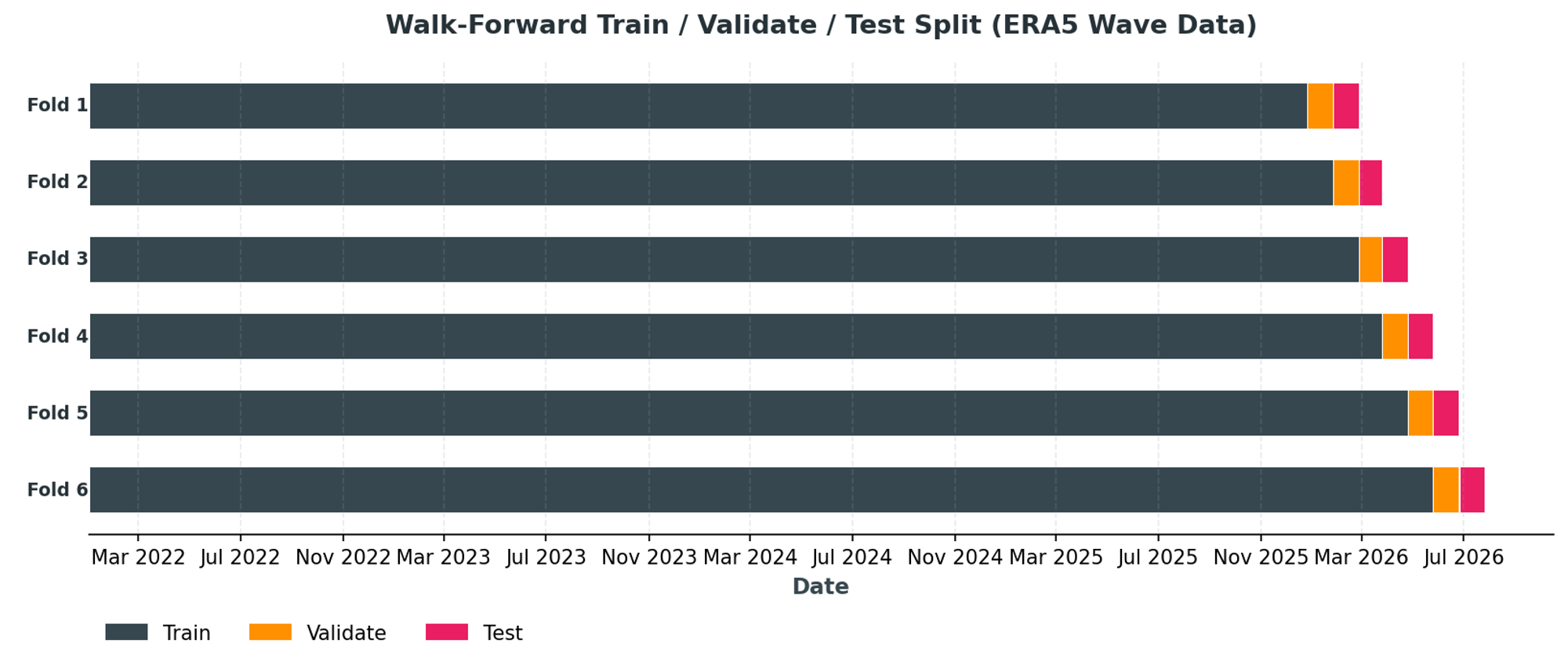
Ordinary k-fold cross-validation shuffles rows at random, which leaks future information into training for a time series. Instead, we use a walk-forward (rolling-origin) split: six folds, each with a one-month validation window and a one-month test window, with training always using everything before that fold’s validation window (an expanding window, not a fixed-size one).
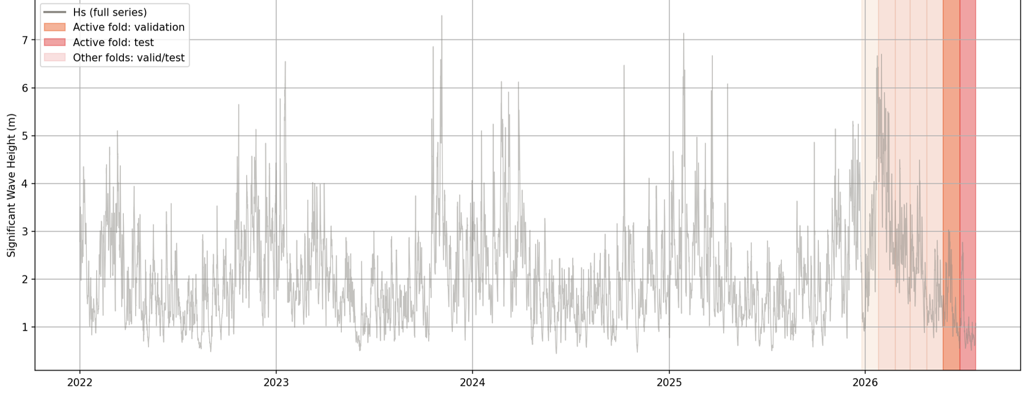
Significant wave height also varies seasonally at this site — smaller, calmer waves in summer (June–August), bigger and stronger swell in winter — which is exactly why a single random split would be risky: it could easily put a disproportionate share of one season into training and the other into test, distorting the evaluation.
2.4 Evaluation Metrics
Five metrics are used to score every (target, lead time) combination:
MAE (Mean Absolute Error):
\[\text{MAE} = \frac{1}{n}\sum_{i=1}^n |y_i - \hat{y}_i|\]RMSE (Root Mean Squared Error):
\[\text{RMSE} = \sqrt{\frac{1}{n}\sum_{i=1}^n (y_i - \hat{y}_i)^2}\]NRMSE (Normalized RMSE), RMSE divided by the range of the actual values, so error magnitude is comparable across targets and lead times that live on different scales (Hs in metres, Te in seconds):
\[\text{NRMSE} = \frac{\text{RMSE}}{\max(y) - \min(y)}\]SMAPE (Symmetric Mean Absolute Percentage Error), used instead of plain MAPE, which is unstable and can blow up whenever the actual value is close to zero. SMAPE is bounded and stable near zero:
\[\text{SMAPE} = \frac{1}{n}\sum_{i=1}^n \frac{|y_i - \hat{y}_i|}{(|y_i| + |\hat{y}_i|)/2}\]R² (Coefficient of Determination):
\[R^2 = 1 - \frac{\sum_i (y_i - \hat{y}_i)^2}{\sum_i (y_i - \bar{y})^2}\]Results
3.1 Optimizing K Features on the Validation Set
Running the recursive feature elimination described above separately for each target and lead time gives the following best feature count and validation-set scores:
| Target | Lead (h) | n_features | RMSE | NRMSE | SMAPE | R² |
|---|---|---|---|---|---|---|
| swh | 1 | 73 | 0.02 | 0.01 | 0.01 | 1.00 |
| swh | 3 | 78 | 0.05 | 0.02 | 0.03 | 0.99 |
| swh | 6 | 78 | 0.11 | 0.05 | 0.06 | 0.96 |
| swh | 12 | 63 | 0.25 | 0.10 | 0.14 | 0.83 |
| swh | 24 | 73 | 0.41 | 0.16 | 0.24 | 0.54 |
| swh | 48 | 108 | 0.54 | 0.22 | 0.31 | 0.20 |
| mwp | 1 | 33 | 0.06 | 0.01 | 0.01 | 1.00 |
| mwp | 3 | 28 | 0.20 | 0.03 | 0.02 | 0.98 |
| mwp | 6 | 33 | 0.41 | 0.06 | 0.04 | 0.92 |
| mwp | 12 | 73 | 0.74 | 0.12 | 0.07 | 0.74 |
| mwp | 24 | 28 | 1.12 | 0.19 | 0.11 | 0.36 |
| mwp | 48 | 8 | 1.28 | 0.22 | 0.14 | 0.05 |
For swh, the optimal feature count stays fairly high across the board and peaks at 108 for the 48h lead. mwp behaves differently: the optimal count actually drops to just 8 features at 48h. That’s not a sign of a cleaner signal — validation R² at that point is only 0.05, essentially no skill — it means additional features had stopped helping a model that had already run out of predictive signal to extract.
3.2 Performance Metrics on the Test Set
Significant wave height (Hs / swh):
| Lead (h) | n_features | MAE | RMSE | NRMSE | SMAPE | R² |
|---|---|---|---|---|---|---|
| 1 | 73 | 0.01 | 0.02 | 0.01 | 0.02 | 1.00 |
| 3 | 78 | 0.04 | 0.06 | 0.02 | 0.04 | 0.99 |
| 6 | 78 | 0.08 | 0.11 | 0.05 | 0.08 | 0.95 |
| 12 | 63 | 0.21 | 0.26 | 0.11 | 0.20 | 0.76 |
| 24 | 73 | 0.38 | 0.42 | 0.19 | 0.35 | 0.36 |
| 48 | 108 | 0.66 | 0.70 | 0.31 | 0.55 | -0.66 |
Mean wave period (Te / mwp):
| Lead (h) | n_features | MAE | RMSE | NRMSE | SMAPE | R² |
|---|---|---|---|---|---|---|
| 1 | 33 | 0.06 | 0.09 | 0.02 | 0.01 | 0.99 |
| 3 | 28 | 0.15 | 0.20 | 0.04 | 0.02 | 0.96 |
| 6 | 33 | 0.33 | 0.42 | 0.09 | 0.05 | 0.81 |
| 12 | 73 | 0.57 | 0.71 | 0.15 | 0.09 | 0.45 |
| 24 | 28 | 0.82 | 1.01 | 0.21 | 0.13 | -0.08 |
| 48 | 8 | 1.01 | 1.25 | 0.26 | 0.16 | -0.63 |
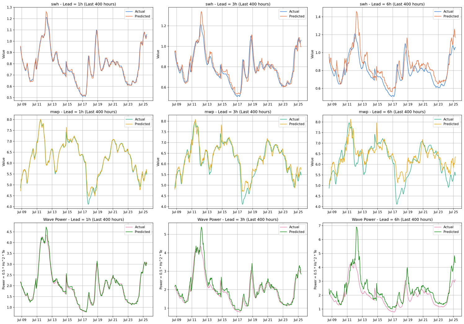
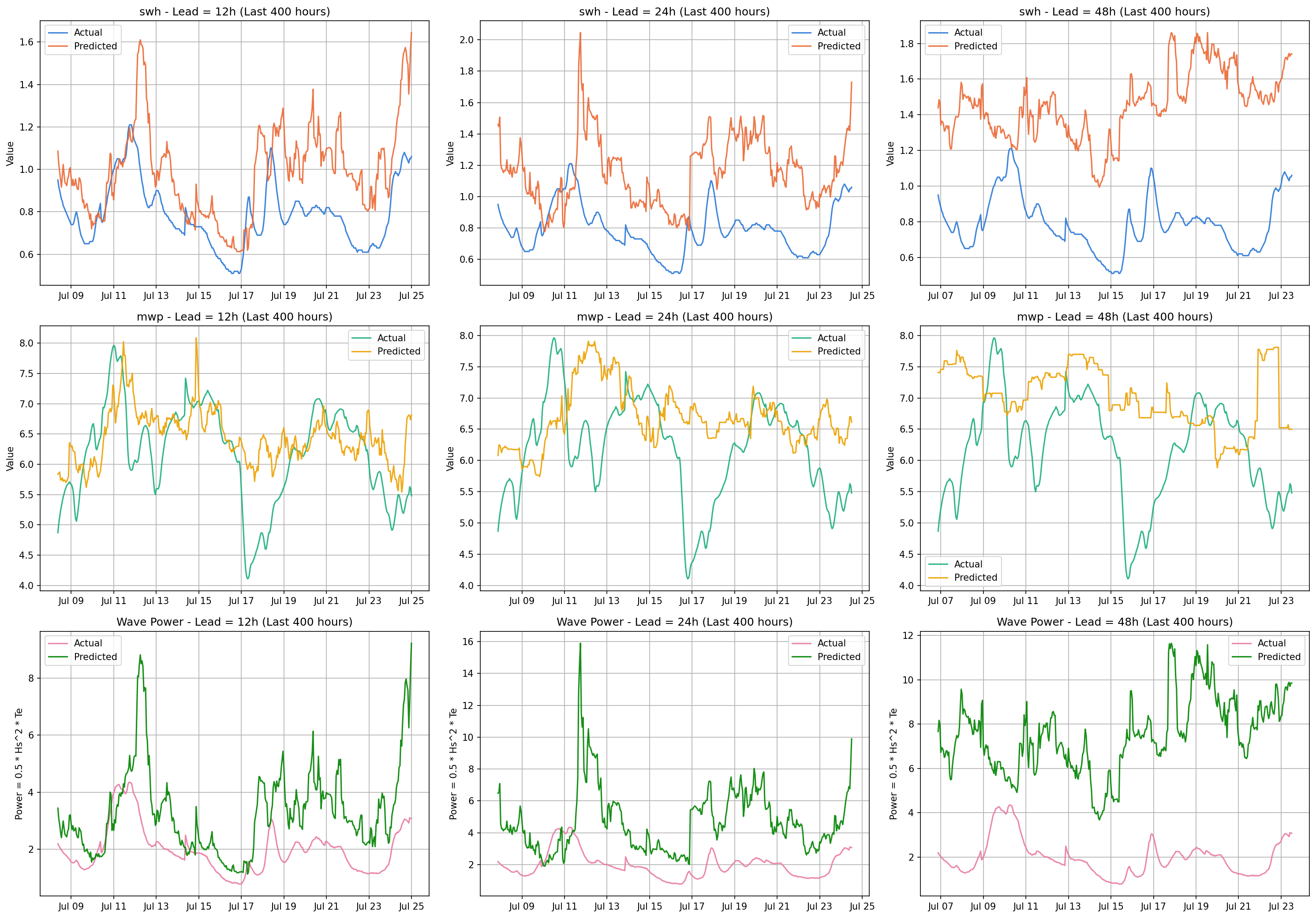
Both targets hold up well through 6h and are still usable at 12h, then degrade sharply. Past 12h, R² keeps falling and actually turns negative for both targets at longer leads (swh at 48h, mwp already by 24h) — worse than just predicting the mean. This isn’t specific to the one test window shown here either: repeating the same evaluation across all six walk-forward folds gives a mean R² of −0.31 (± 0.35) for swh and −0.11 (± 0.22) for mwp at 48h, so it’s a consistent property of the model at that lead, not a fluke of which month landed in the test set. Hs is consistently the easier target to forecast — its R² stays above mwp’s at every lead time up to 24h.
3.3 Time Series Forecasting
The model performs well before the 12h lead time; after that, bias grows noticeably higher. SWH prediction is also consistently better than MWP.
Simplifications
- Hs and Te are forecast independently, as two separate LightGBM models, and only combined into a wave power estimate afterward. Errors in each compound multiplicatively in the derived power series.
- The power formula uses the rounded coefficient 0.5, not the more precise 0.49 physical constant, throughout the diagnostic plots and the derived power series.
- A single walk-forward fold is shown in the results tables and figures above (the most recent of six); the fold-averaged R² quoted in Section 3.2 is the only place all six are used together.
- Purely autoregressive. The feature set is built entirely from lags of the ERA5 variables themselves, with no coupled physical wave model in the loop — a likely contributor to the sharp skill drop-off beyond a 12h lead.
Conclusion
An autoregressive LightGBM model, fed lagged ERA5 ocean variables and cyclical time encodings, forecasts significant wave height and mean wave period well up to a 6–12h lead, and loses real skill beyond that — R² for both targets turns negative by 24–48h, consistently across all six walk-forward folds. Part 2 moves to a multi-model stacking ensemble (Ridge Regression, Random Forest, and LightGBM) to see whether combining model families recovers some of that longer-lead skill.
References
Code
- LightGBM_ERA5_3.py: data loading, walk-forward fold construction, feature engineering, RFE feature selection, final model training, and all figures above.
- ERA5_Ocean_2024_01_to_2026_07.csv: the raw ERA5 hourly ocean data pulled from the Climate Data Store.
Results_3/folder: best feature count per lead time, test-set metrics, and the six-fold walk-forward summary.
Next: Part 3 (numbering continues from the series) will stack Ridge Regression, Random Forest, and LightGBM together and check whether the ensemble holds up better than LightGBM alone at longer lead times.
M. Wang, F. Ying, and J. Jia, “Ocean wave power flux forecasting using a stacking ensemble of LSTM and LightGBM,” Renewable Energy, vol. 256, p. 124597, 2026. ↩