Stochastic Optimisation for Energy Storage (Part 2)
Published:
Series: Stochastic Optimisation for Energy Storage Part: 2 (Implementation)
Part 1 laid out the theory: a two-stage stochastic program commits a first-stage decision before the uncertain outcome is known, then evaluates it against however many possible outcomes are being planned against. This post turns that into working code: a real battery dispatch problem, solved in Pyomo, with the scenario set built from real quantile forecasts rather than the six hand-picked historical days used in the earlier Storage_Dispatch series.
Overview
Three pieces come together here. The quantile forecasting machinery from PEPF Part 2 generates the price scenarios. The battery physics are the same assumed specification used throughout this project. The dispatch problem connecting them is formulated exactly as the two-stage program from Part 1, and solved with Pyomo instead of a hand-written linear program.
The result is compared against two baselines on a real, held-out test day: a naive schedule that trusts only the median forecast, and a perfect-foresight schedule that cheats by seeing the actual realized prices. That comparison is the actual point of a two-stage stochastic model, not the theory alone.
Turning Quantile Forecasts Into Scenarios
The target day is 10 July 2025. The forecast origin is set to noon the day before, 9 July 2025, matching when a real day-ahead auction closes. Everything the model is allowed to use must be known by that point.
For every hour of the target day, a separate Quantile Regression model is trained (reusing the feature engineering from PEPF Part 2: calendar features plus price lags) on all data before the forecast origin, and used to predict five quantile levels: 0.10, 0.30, 0.50, 0.70, and 0.90. Fixing the same quantile level across all 24 hours gives one internally consistent price path per level, the “low” scenario runs low all day, the “median” scenario runs at the median all day, and so on. This is a standard simplification for turning independent hourly quantiles into a joint scenario set. Each of the five scenarios gets equal probability (0.2), since the levels are evenly spaced.
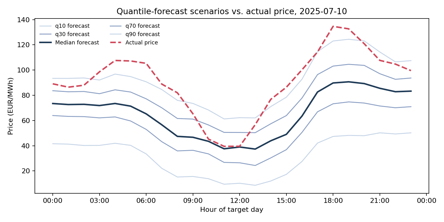 The five scenario paths built for 10 July 2025, against the price that actually happened. The forecast band captures the midday trough well but is exceeded by the actual price during the early-morning and evening peaks.
The Two-Stage Dispatch Model
The first-stage decision is the battery’s full charge and discharge schedule for the day, one shared schedule across every scenario, since the battery physically has to commit to a schedule before delivery. The second-stage “decision” here is simple: realized profit under whichever scenario turns out to hold. There is no intraday recourse in this version; that simplification is discussed below.
m.pc = pyo.Var(m.T, bounds=(0, p_max))   # charging power, shared across scenarios
m.pd = pyo.Var(m.T, bounds=(0, p_max))   # discharging power, shared across scenarios
m.soc = pyo.Var(m.T, bounds=(e_min, e_max))

def soc_rule(m, t):
    prev = e0 if t == 0 else m.soc[t - 1]
    return m.soc[t] == prev + eta_c * m.pc[t] - m.pd[t] / eta_d
m.soc_con = pyo.Constraint(m.T, rule=soc_rule)

expected_profit = sum(
    probabilities[s] * sum(scenario_prices[s][t] * (m.pd[t] - m.pc[t]) for t in range(HOURS))
    for s in scenarios
)
m.obj = pyo.Objective(expr=expected_profit, sense=pyo.maximize)
The same model, solved with a single scenario instead of five, produces both baselines: the naive schedule uses only the median forecast path, and the perfect-foresight schedule uses the actual realized prices.
Battery Assumptions
The battery specification is unchanged from Storage_Dispatch_part2: a stated hypothesis, not a measurement.
| Parameter | Value |
|---|---|
| Rated power | 1 MW |
| Usable capacity | 2 MWh |
| State-of-charge range | 10% to 90% |
| Charge / discharge efficiency | 95% each way |
| Starting charge | 50% |
Results and Discussion
All three schedules are evaluated on the actual realized price for 10 July 2025.
| Schedule | Realized profit |
|---|---|
| Stochastic (5 scenarios) | €193.60 |
| Naive (median forecast) | €200.77 |
| Perfect foresight | €227.67 |
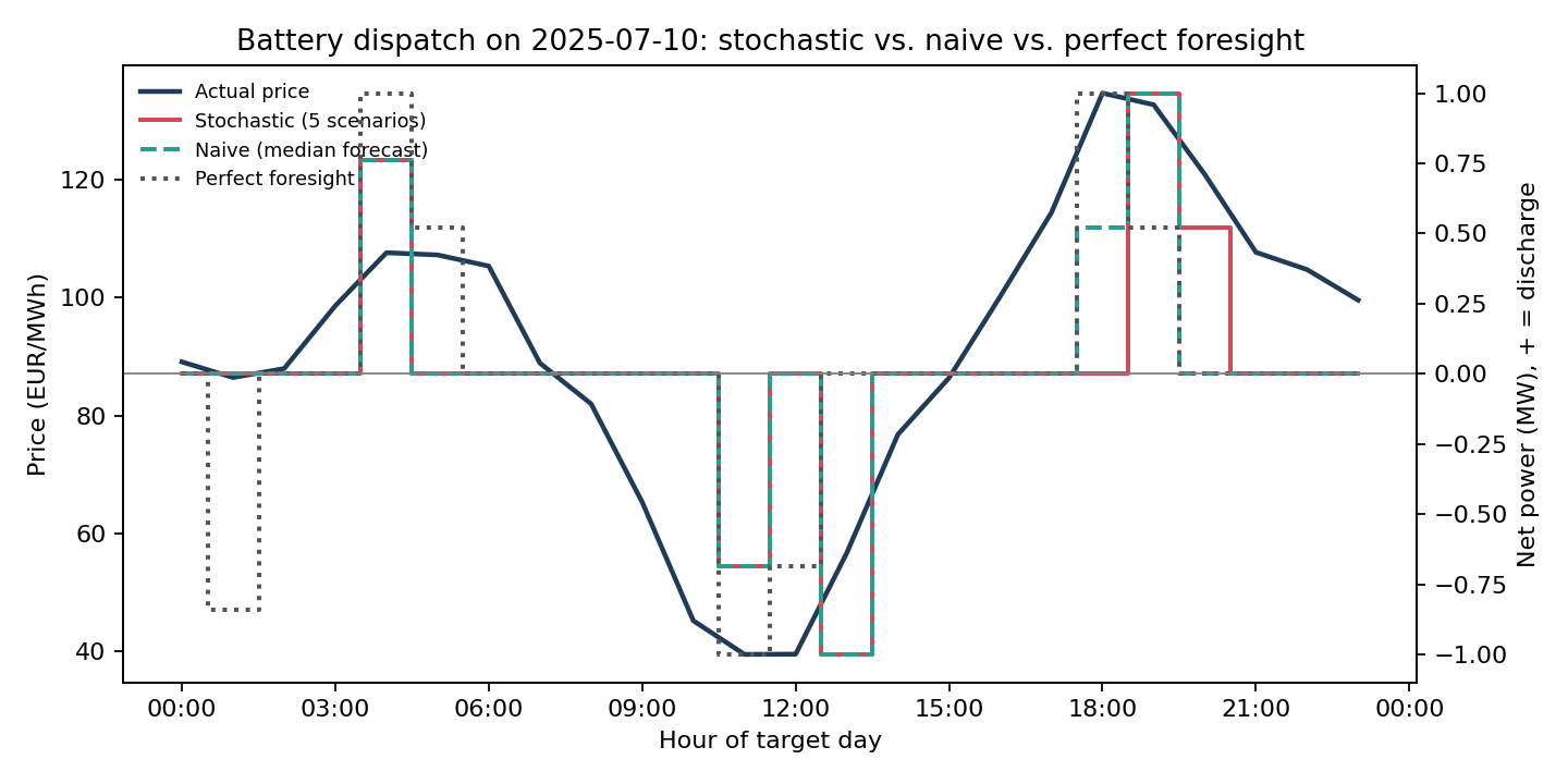 All three schedules charge in the same two windows and discharge into the same two price peaks; the stochastic and naive schedules differ only by a one-hour shift in when the evening discharge happens.
The stochastic schedule made €7.17 less than the naive median-only schedule on this particular day, a negative result for the stochastic approach, and worth reporting exactly as it came out rather than picking a friendlier test day. The dispatch comparison plot shows why: the two schedules are nearly identical. Both charge overnight and again through the midday trough, and both discharge into the morning and evening price peaks. The only real difference is that the stochastic schedule’s evening discharge lands one hour later than the naive one, and the actual price had already started falling by then, turning a small timing difference into a small loss.
This happened because the five scenarios do not disagree much about when the day’s peaks and troughs occur, only about their size. Fixing the same quantile level across every hour, by construction, preserves the median forecast’s timing in every scenario; it only stretches or compresses the price level around that timing. When the schedules barely disagree on timing, weighting five similar-shaped scenarios cannot outperform trusting the single median path, and a one-hour difference in either direction is within the noise of which one wins on a single test day.
The gap to perfect foresight is more informative: €34.08, about 15% of the perfect-foresight profit. That gap is not a modeling failure to fix, it is the actual, honest cost of not knowing the future, and the figure above shows exactly where it comes from: perfect foresight charges during the very cheapest early-morning hours (00:00 to 02:00), a window none of the five scenarios flagged as unusually cheap, because the actual price dipped there while every quantile forecast expected a flatter overnight profile.
Simplifications
A few things a fuller model would include were deliberately left out.
- Comonotonic scenarios. Fixing the same quantile level across all 24 hours is a simplification; it cannot represent a scenario where the morning is cheap but the evening surprises high, since real hour-to-hour forecast errors are correlated but not perfectly so.
- No intraday recourse. The schedule is committed once for the whole day. A real operator can adjust through the intraday market as the day unfolds; that would make this a genuine multi-stage problem rather than a two-stage one.
- Five scenarios, not a full lattice. Wimmeder (2021) works with the full apparatus of scenario lattices and approximate dual dynamic programming for exactly this reason, five comonotonic paths is a coarse approximation to the true joint distribution.
- One test day. A single day proves very little on its own; the loss reported here easily could have gone the other way on a different day, which is the entire reason walk-forward validation exists elsewhere in this project.
Conclusion
The two-stage stochastic model from Part 1 now runs on real data: real quantile forecasts build the scenarios, and Pyomo solves the dispatch. On this one test day, the stochastic schedule did not beat a naive median-only schedule, and the reason was traceable rather than mysterious, the scenarios agreed on timing and differed only on price level, leaving little for a weighted schedule to exploit. The more useful number was the 15% gap to perfect foresight, which is the honest cost of forecasting under uncertainty rather than a bug to fix. Closing that gap further would need scenarios that can disagree on timing, not just magnitude, and a schedule that can react intraday rather than committing once.
References
- Wimmeder, S. (2021). Stochastic Optimization of a Battery Storage System. Master’s thesis, TU Wien, in cooperation with the Austrian Institute of Technology. Section 3.6 discusses the value of the stochastic solution referenced above.
- Probabilistic Electricity Price Forecasting (Part 2) — the Quantile Regression pipeline reused here to build the scenario set.
Code
- Data.csv: the same DK1 price and generation-mix data used throughout the PEPF and Storage Dispatch series, sourced from Energi Data Service.
- qr_qrf_walkforward_pipeline.py: data loading, feature engineering, and the Quantile Regression fitting code, reused unchanged from PEPF Part 2.
- stochastic_battery_dispatch.py: builds the scenarios, defines and solves the Pyomo two-stage dispatch model, and produces the figures and CSVs above.
Results/folder: dispatch schedules and the profit summary.
Next: Part 3 will add a genuine multi-stage recourse structure, letting the schedule adjust through the day rather than committing once at the forecast origin.