Probabilistic Electricity Price Forecasting (Part 2)
Published:
Series: Probabilistic Electricity Price Forecasting Part: 2 (Implementation and Results)
This post develops QR and QRF using the same data source, Energi Data Service, with a clean date range from 2024-01-01 to 2025-09-30 UTC, excluding subsequent empty and unreported price periods, and incorporating the same post-production exogenous features.
That window covers 639 days, or 15,336 hourly observations.
1. Data and Features
TARGET   = "DK1_EUR/MWh"
DATE_COL = "HourUTC"

FEATURE_COLS = [
    "LocalPowerMWhDK1",
    "LocalPowerSelfConMWhDK1",
    "CentralPowerMWhDK1",
    "CommercialPowerMWhDK1",
    "HydroPowerMWhDK1",
    "OffshoreWindGe100MW_MWhDK1",
    "OffshoreWindLt100MW_MWhDK1",
    "OnshoreWindGe50kW_MWhDK1",
    "OnshoreWindLt50kW_MWhDK1",
    "SolarPowerGe10Lt40kW_MWhDK1",
    "SolarPowerGe40kW_MWhDK1",
    "SolarPowerLt10kW_MWhDK1",
    "SolarPowerSelfConMWhDK1",
    "PowerToHeatMWhDK1",
    "GrossConsumptionMWhDK1",
]
| Feature Name | Full Form / Category | Description |
|---|---|---|
| DK1_EUR/MWh | DK1 Electricity Spot Price | Hourly elspot price in the DK1 zone (€/MWh). |
| LocalPowerMWhDK1 | Local Power Production | Electricity generated by local power plants (MWh). |
| LocalPowerSelfConMWhDK1 | Local Power Self-Consumption | Locally produced electricity consumed without entering the grid (MWh). |
| CentralPowerMWhDK1 | Central Power Production | Electricity generated by large centralized power plants (MWh). |
| CommercialPowerMWhDK1 | Commercial Power Production | Electricity produced for commercial purposes, often by private operators (MWh). |
| HydroPowerMWhDK1 | Hydropower Production | Electricity generated from hydroelectric plants in DK1 (MWh). |
| OffshoreWindGe100MW_MWhDK1 | Offshore Wind (≥100 MW) | Electricity generated by offshore wind farms ≥100 MW (MWh). |
| OffshoreWindLt100MW_MWhDK1 | Offshore Wind (<100 MW) | Electricity generated by offshore wind farms <100 MW (MWh). |
| OnshoreWindGe50kW_MWhDK1 | Onshore Wind (≥50 kW) | Electricity generated by onshore wind farms ≥50 kW (MWh). |
| OnshoreWindLt50kW_MWhDK1 | Onshore Wind (<50 kW) | Electricity generated by small onshore wind farms <50 kW (MWh). |
| SolarPowerGe10Lt40kW_MWhDK1 | Solar Power (10–40 kW) | Solar electricity generated from systems between 10–40 kW (MWh). |
| SolarPowerGe40kW_MWhDK1 | Solar Power (>40 kW) | Solar electricity generated from systems >40 kW (MWh). |
| SolarPowerLt10kW_MWhDK1 | Solar Power (<10 kW) | Solar electricity from small residential or business systems <10 kW (MWh). |
| SolarPowerSelfConMWhDK1 | Solar Power Self-Consumption | Solar power generated and consumed on-site without exporting to the grid (MWh). |
| PowerToHeatMWhDK1 | Power-to-Heat Conversion | Electricity converted to heat, often for district heating systems (MWh). |
| GrossConsumptionMWhDK1 | Gross Electricity Consumption | Total electricity consumed, including losses and self-consumption (MWh). |
2. Building the QR and QRF Pipeline
The earlier theory post committed to two models: Quantile Regression (QR) and Quantile Regression Forest (QRF). This section walks through the actual implementation, step by step, and evaluates both on the DK1 data above using walk-forward cross-validation rather than a single train/test split. The full pipeline is split across qr_qrf_walkforward_pipeline.py (data, models, evaluation) and forecasting_plots.py (all figures), both included alongside this post.
2.1 Feature Engineering
Each row needs calendar features (hour, day of week, month) and lagged price features. The lags are built relative to the forecast lead time $L$, so a model trained for the 6h-ahead task only ever sees information that would actually be available 6 hours before delivery:
df["hour"] = df[DATE_COL].dt.hour
df["dayofweek"] = df[DATE_COL].dt.dayofweek
df["month"] = df[DATE_COL].dt.month
df["is_weekend"] = (df["dayofweek"] >= 5).astype(int)
df["is_peak"] = df["hour"].between(7, 20).astype(int)

# Lag features relative to lead time L
df[f"price_lag_{L}"] = df[TARGET].shift(L)
df[f"price_lag_{L + 24}"] = df[TARGET].shift(L + 24)
df["price_lag_168"] = df[TARGET].shift(168)
df["price_rolling_24h"] = df[TARGET].shift(L).rolling(24).mean()
df = df.dropna().reset_index(drop=True)
price_lag_168 is last week’s price at the same hour; price_rolling_24h is a 24-hour rolling average ending at the last point actually known before the target.
2.2 Walk-Forward Train / Validate / Test Split
A single chronological split (train on everything before a cutoff, test on what’s after) only tells us how the model does on one slice of time. DK1 prices are seasonal and regime-dependent, so this project instead uses walk-forward, expanding-window cross-validation: four folds, spread across the full 2024 to 2025 timeline, each with its own Train, then Validate, then Test window, in that order:
def generate_walk_forward_folds(min_date, max_date, n_folds, test_len_h, val_len_h, min_train_frac):
    total_hours = (max_date - min_date) / pd.Timedelta(hours=1)
    min_train_len = total_hours * min_train_frac
    remaining = total_hours - min_train_len
    step = remaining / n_folds

    folds = []
    for k in range(n_folds):
        val_start = min_date + pd.Timedelta(hours=min_train_len + k * step)
        val_end = val_start + pd.Timedelta(hours=val_len_h)
        test_start = val_end
        test_end = min(test_start + pd.Timedelta(hours=test_len_h), max_date)
        folds.append(dict(
            fold=k + 1,
            train_start=min_date, train_end=val_start,
            val_start=val_start, val_end=val_end,
            test_start=test_start, test_end=test_end,
        ))
    return folds
Training always starts from the same date and expands; validation and test windows are spaced evenly across the remaining timeline, so each fold lands in a different season:
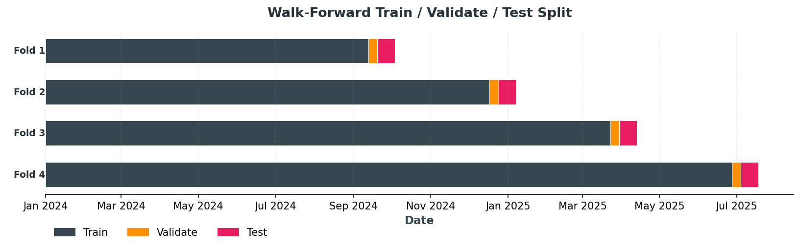 The four walk-forward folds actually used. Fold 2’s test window falls over Christmas and New Year; the others fall in early autumn, early spring, and midsummer.
The validation window is not just a formality: it’s where QRF’s min_samples_leaf is chosen (between 20 and 40, by whichever gives the lower validation pinball loss) before either model ever sees the test window.
2.3 Fitting Quantile Regression
QR fits one linear model per quantile level, each minimizing the pinball loss directly rather than the squared error. An earlier version of this pipeline used sklearn’s QuantileRegressor, which solves this as a linear program and turned out to scale badly: about 20 seconds per quantile on this project’s larger folds. Switching to statsmodels’ QuantReg, which uses iteratively reweighted least squares instead of a linear program, cut that to roughly 1 to 4 seconds per quantile, for the same result:
import statsmodels.api as sm
from statsmodels.regression.quantile_regression import QuantReg
from sklearn.preprocessing import StandardScaler

QUANTILES = [0.025, 0.05, 0.10, 0.20, 0.30, 0.40, 0.50, 0.60, 0.70, 0.80, 0.90, 0.95, 0.975]

def fit_quantile_regression_models(X_train, y_train, quantiles, max_iter=1000, p_tol=1e-6):
    scaler = StandardScaler()
    X_train_s = scaler.fit_transform(X_train)
    X_train_c = sm.add_constant(X_train_s, has_constant="add")

    models = {}
    for a in quantiles:
        models[a] = QuantReg(y_train, X_train_c).fit(q=a, max_iter=max_iter, p_tol=p_tol)
    return {"scaler": scaler, "models": models}


def predict_quantile_regression(fitted, X):
    X_c = sm.add_constant(fitted["scaler"].transform(X), has_constant="add")
    return {a: np.asarray(res.predict(X_c)) for a, res in fitted["models"].items()}
The models are fit once per fold, on the training window only, then reused to predict on both the validation and test windows, rather than refitting from scratch for each.
Because each quantile is fit independently, nothing stops the 0.90 line from occasionally landing below the 0.80 line, a problem called quantile crossing. The standard fix is to sort the predicted quantiles row by row after the fact:
def enforce_monotonicity(preds, quantiles):
    sorted_q = np.sort(quantiles)
    stacked = np.vstack([preds[a] for a in sorted_q])
    before_cross = float(np.mean(np.any(np.diff(stacked, axis=0) < 0, axis=0)))
    stacked_sorted = np.sort(stacked, axis=0)
    fixed = {a: stacked_sorted[k] for k, a in enumerate(sorted_q)}
    return fixed, before_cross
before_cross is kept as a diagnostic: it reports how often crossing actually happened before the fix, which turns out to be a useful signal on its own (see Section 3.5 below).
2.4 Fitting Quantile Regression Forest
QRF follows the Meinshausen algorithm from the theory post exactly: grow a standard Random Forest, but instead of collapsing each leaf to its mean, keep every training sample that lands there. At prediction time, each tree assigns a weight to every training point depending on whether it shares a leaf with the query point; averaging these weights across trees gives the forest-weighted empirical CDF, and inverting it gives the quantile.
The first version of this class predicted one test row at a time, looping over every tree in Python, a real bottleneck once it had to run across four folds and four lead times. It’s now vectorized with sparse matrices: for each tree, leaf membership becomes a one-hot matrix, weights for the whole test set are computed in a single sparse matrix multiplication per tree, and the final quantile lookup runs as one batched cumulative sum over the entire test set instead of a per-row loop:
from scipy import sparse
from sklearn.ensemble import RandomForestRegressor

class QuantileRandomForest:
    def __init__(self, n_estimators=200, min_samples_leaf=30, random_state=42, n_jobs=-1):
        self.rf = RandomForestRegressor(
            n_estimators=n_estimators, min_samples_leaf=min_samples_leaf,
            random_state=random_state, n_jobs=n_jobs,
        )

    def fit(self, X, y):
        self.y_train_ = np.asarray(y)
        self.rf.fit(X, self.y_train_)
        self.train_leaves_ = self.rf.apply(X)  # (n_train, n_trees)
        self.n_trees_ = self.train_leaves_.shape[1]
        self.n_train_ = X.shape[0]
        return self

    def _tree_weight_matrix(self, t, test_leaf_ids):
        train_leaf_ids = self.train_leaves_[:, t]
        leaves, train_inv = np.unique(train_leaf_ids, return_inverse=True)
        train_onehot = sparse.csr_matrix(
            (np.ones(self.n_train_, dtype=np.float32), (np.arange(self.n_train_), train_inv)),
            shape=(self.n_train_, len(leaves)),
        )
        leaf_counts = np.asarray(train_onehot.sum(axis=0)).ravel()
        inv_counts = np.divide(1.0, leaf_counts, out=np.zeros_like(leaf_counts), where=leaf_counts > 0)
        train_onehot_norm = train_onehot.multiply(inv_counts).tocsr()

        leaf_to_col = {leaf: i for i, leaf in enumerate(leaves)}
        test_col = np.fromiter((leaf_to_col.get(l, -1) for l in test_leaf_ids), dtype=int, count=len(test_leaf_ids))
        valid = test_col >= 0
        test_onehot = sparse.csr_matrix(
            (np.ones(int(valid.sum()), dtype=np.float32), (np.where(valid)[0], test_col[valid])),
            shape=(len(test_leaf_ids), len(leaves)),
        )
        return test_onehot @ train_onehot_norm.T  # (n_test, n_train), sparse

    def predict_quantiles(self, X, quantiles):
        test_leaves = self.rf.apply(X)
        W = sparse.csr_matrix((X.shape[0], self.n_train_), dtype=np.float32)
        for t in range(self.n_trees_):
            W = W + self._tree_weight_matrix(t, test_leaves[:, t])
        W = (W / self.n_trees_).toarray().astype(np.float32)

        order = np.argsort(self.y_train_)
        y_sorted, cdf = self.y_train_[order], np.cumsum(W[:, order], axis=1)
        cdf[:, -1] = 1.0  # guard against floating-point residue

        return {a: y_sorted[np.argmax(cdf >= a, axis=1)] for a in quantiles}
Unlike QR, QRF is monotonic by construction: the quantiles are all read off the same weighted CDF, so a higher $\alpha$ can never produce a lower value. min_samples_leaf is selected per fold from {20, 40} using the validation window described in 2.2.
2.5 Evaluation Metrics, Averaged Across Folds
Both models are scored with the same metrics introduced in the theory post: mean pinball loss, the CRPS approximation (twice the average pinball loss over the grid), empirical coverage, and mean interval width (upper quantile minus lower quantile, in €/MWh) for the 80/90/95% intervals. With four folds instead of one split, each metric is now reported as a mean across folds, with a standard deviation showing how much it varies fold to fold:
def pinball_loss(y_true, q_hat, alpha):
    err = y_true - q_hat
    return float(np.mean(np.where(err >= 0, alpha * err, (alpha - 1) * err)))

def crps_from_pinball(y_true, quantile_preds, quantiles):
    losses = [pinball_loss(y_true, quantile_preds[a], a) for a in quantiles]
    return 2.0 * np.mean(losses), np.mean(losses)

def empirical_coverage(y_true, lower, upper):
    return float(np.mean((y_true >= lower) & (y_true <= upper)))
The pipeline runs both models across four lead times (1h, 6h, 12h, 24h) and all four folds, then aggregates.
3. Results and Discussion
In one sentence: QRF is more accurate and better calibrated than QR at almost every lead time, but both models’ calibration collapses during unusual weeks like holidays, a failure only walk-forward validation reveals.
Running qr_qrf_walkforward_pipeline.py on the real DK1 data, across all four walk-forward folds, gives the results below. Each number is the mean across the 4 folds, with the standard deviation in parentheses showing how much that metric actually varies from one time period to the next.
A useful way to judge any probabilistic forecast: check accuracy first, then whether the stated uncertainty can be trusted (calibration), then how tight it is (sharpness), and finally combine the last two into one verdict, since neither alone tells the full story. The subsections below follow exactly that order.
3.1 Accuracy
| Model | Lead Time | MAE (median) | RMSE (median) | Mean Pinball | CRPS (approx.) |
|---|---|---|---|---|---|
| QR | 1h | 11.16 (±2.51) | 16.04 (±4.70) | 3.53 (±0.73) | 7.07 (±1.46) |
| QRF | 1h | 8.55 (±2.43) | 13.46 (±4.65) | 2.74 (±0.66) | 5.47 (±1.32) |
| QR | 6h | 20.09 (±3.44) | 25.37 (±3.38) | 6.35 (±1.39) | 12.70 (±2.78) |
| QRF | 6h | 17.83 (±3.91) | 24.44 (±4.12) | 5.55 (±1.35) | 11.10 (±2.70) |
| QR | 12h | 20.89 (±3.94) | 26.14 (±4.25) | 6.48 (±1.55) | 12.95 (±3.09) |
| QRF | 12h | 17.88 (±3.91) | 24.49 (±4.07) | 5.49 (±1.26) | 10.98 (±2.51) |
| QR | 24h | 20.63 (±2.96) | 25.96 (±3.94) | 6.39 (±1.33) | 12.77 (±2.65) |
| QRF | 24h | 16.19 (±2.53) | 22.21 (±2.87) | 4.89 (±0.69) | 9.77 (±1.38) |
QRF wins on every metric at every lead time (24h: MAE 16.19 vs 20.63 €/MWh, CRPS 9.77 vs 12.77 €/MWh), but the size of the win isn’t uniform:
| Lead time | MAE reduction | RMSE reduction | Mean pinball reduction | CRPS reduction |
|---|---|---|---|---|
| 1h | 23% | 16% | 22% | 23% |
| 6h | 11% | 4% | 13% | 13% |
| 12h | 14% | 6% | 15% | 15% |
| 24h | 21% | 14% | 24% | 23% |
Gains are largest at 1h and 24h (14 to 24%, depending on the metric) and noticeably smaller at 6h and 12h (4 to 15%), the same two horizons where QRF’s own calibration turns out to be shakiest below. That’s not a coincidence. Whatever makes mid-horizon forecasting hard (regime shifts, a weaker lag signal) also caps how much QRF’s extra flexibility can buy.
Two things follow. First, the RMSE gap (driven by large errors) is close to the MAE gap at every horizon, so QRF isn’t just nudging the median, it’s handling spikes better, consistent with a forest picking up nonlinearities and tail behaviour a linear model per quantile can’t. Second, the CRPS gap tracks the pinball gap almost exactly, confirming QRF’s whole predictive CDF sits closer to the empirical distribution, not just a couple of quantiles that happen to look good. But accuracy alone says nothing about whether the model’s stated uncertainty can be trusted, that’s next.
3.2 Calibration and Sharpness
Does the stated interval actually catch the outcome as often as promised (calibration), and how tight is it while doing so (sharpness)? A narrow interval that misses often isn’t sharper, it’s just wrong more confidently, so the two have to be read together.
| Model | Lead Time | Cov 80% (nom. 0.80) | Width 80% | Cov 90% (nom. 0.90) | Width 90% | Cov 95% (nom. 0.95) | Width 95% |
|---|---|---|---|---|---|---|---|
| QR | 1h | 0.815 (±0.070) | 38.2 | 0.910 (±0.029) | 54.2 | 0.955 (±0.015) | 68.1 |
| QRF | 1h | 0.862 (±0.061) | 31.4 | 0.926 (±0.042) | 43.8 | 0.965 (±0.028) | 56.1 |
| QR | 6h | 0.735 (±0.166) | 58.5 | 0.809 (±0.152) | 77.9 | 0.868 (±0.120) | 97.1 |
| QRF | 6h | 0.727 (±0.157) | 48.0 | 0.844 (±0.129) | 65.2 | 0.919 (±0.073) | 83.3 |
| QR | 12h | 0.738 (±0.165) | 59.5 | 0.802 (±0.155) | 76.0 | 0.855 (±0.130) | 94.3 |
| QRF | 12h | 0.726 (±0.135) | 47.9 | 0.851 (±0.102) | 65.1 | 0.927 (±0.058) | 82.7 |
| QR | 24h | 0.721 (±0.176) | 56.8 | 0.820 (±0.138) | 74.7 | 0.889 (±0.080) | 94.0 |
| QRF | 24h | 0.781 (±0.073) | 48.9 | 0.898 (±0.044) | 65.7 | 0.952 (±0.022) | 82.8 |
QRF is narrower than QR at every lead time (24h, 90% interval: 65.7 vs 74.7 €/MWh), with calibration that’s comparable at 1h and clearly better from 6h onward. The coverage deltas (empirical − nominal) make that pattern precise:
| Cov80 delta | Cov90 delta | Cov95 delta | |
|---|---|---|---|
| QR, 1h | +0.015 | +0.010 | +0.005 |
| QRF, 1h | +0.062 | +0.026 | +0.015 |
| QR, 6h | −0.065 | −0.091 | −0.082 |
| QRF, 6h | −0.073 | −0.056 | −0.031 |
| QR, 12h | −0.062 | −0.098 | −0.095 |
| QRF, 12h | −0.074 | −0.049 | −0.023 |
| QR, 24h | −0.079 | −0.080 | −0.061 |
| QRF, 24h | −0.019 | −0.002 | +0.002 |
At 1h, both models are slightly conservative (small positive deltas). At 6h and 12h, QR’s deltas run as large as −0.10. QRF’s 90% and 95% intervals improve noticeably there, but its 80% interval doesn’t (−0.073 to −0.074, marginally worse than QR’s), so “QRF calibrates better at mid-horizons” is only half true. It depends which interval you’re looking at. By 24h, QRF is essentially on target while QR is still under-covering by 6 to 8 points.
Averaged across folds these gaps look moderate, mostly a few points off nominal. But the average hides real fold-to-fold collapse. The reported ± is the standard deviation across the four folds, and it’s large: QR’s Cov80 at 6h is 0.735 (±0.166), meaning individual folds swing roughly ±16 percentage points around that mean. Two of the four folds are consistently the hardest to calibrate for both models. Fold 1 (test window 19 September to 3 October 2024) and Fold 3 (30 March to 13 April 2025) calibrate well, close to nominal coverage at every lead time. Fold 2 (24 December 2024 to 7 January 2025, spanning Christmas and New Year) and Fold 4 (4 to 18 July 2025) collapse to 53–66% actual coverage against an 80% nominal target. Reporting only the fold-average, the way a single train/test split effectively forces you to, hides that collapse entirely.
Is a collapse like that statistically real, or just noise from a small test window? For a fold with $T_f$ test points, treat coverage as a binomial proportion and build a 95% confidence interval around the empirical estimate $\hat C$:
\[\hat C \pm 1.96\sqrt{\frac{\hat C(1-\hat C)}{T_f}}\]With a two-week test window ($T_f \approx 336$ hours) and a fold where coverage drops to $\hat C = 0.55$ against an 80% target: $0.55 \pm 1.96\sqrt{0.55 \times 0.45 / 336} \approx 0.55 \pm 0.053$, or roughly $[0.50, 0.60]$. Nominal 0.80 sits far outside that band, so this is a genuinely miscalibrated fold, not sampling noise.
Combining calibration and sharpness is the actual verdict, not either metric alone:
| Width | Coverage | Verdict | What it means |
|---|---|---|---|
| Narrow | Matches nominal | Excellent | The interval is both tight and honest: it claims high confidence and earns it. Nothing to fix. |
| Narrow | Below nominal | Overconfident | The interval is tight, but the outcome falls outside it more often than promised. It’s making a confident claim it can’t back up, the worst combination, since it looks precise while actually misleading. |
| Wide | Above nominal | Underconfident (too cautious) | The interval catches the outcome more often than it needs to, but only because it’s wider than necessary. Safe, but not sharp, there’s room to tighten it without losing reliability. |
| Wide | Matches nominal | Conservative but calibrated | The interval is wider than it strictly needs to be, but it’s honest about it: the stated confidence level is met. Trustworthy, just not efficient. |
QRF sits closest to the narrow-and-matching cell for most lead times, which is why it’s the model to reach for by default; QR is both wider and, on its worst folds, still under-covering, the less favourable combination of the two.
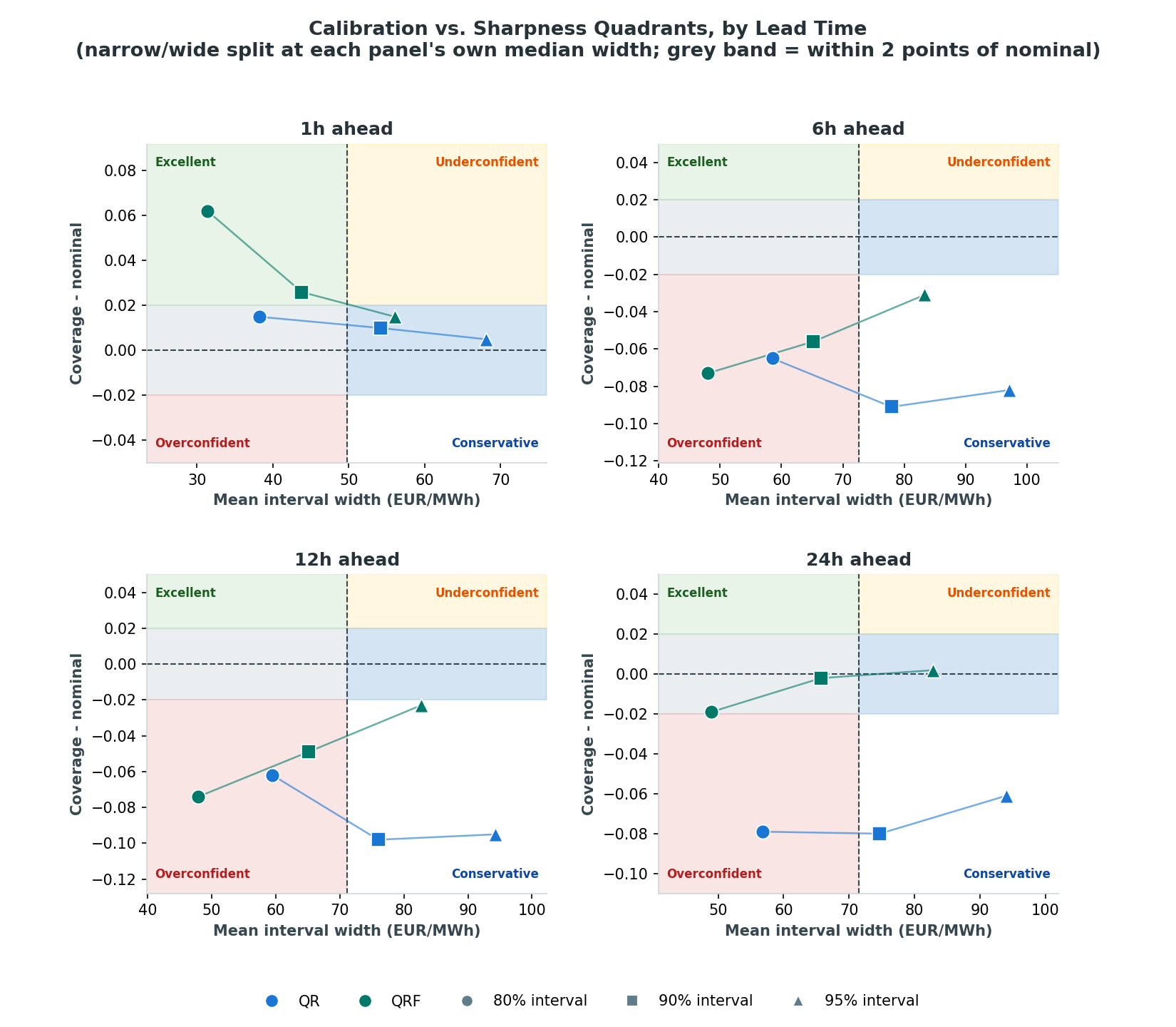 Each panel plots mean interval width against coverage minus nominal, for QR and QRF at the 80/90/95% levels, at one lead time. QRF (teal) sits in or near the Excellent quadrant at 1h and drifts toward it by 24h; QR (blue) sits mostly in Overconfident at 6h through 24h, wider than QRF and still under-covering.
A rough grading scale. There’s no official standard for what counts as a “good” pinball loss, CRPS, or coverage gap; it depends on price volatility and the specific market. As a reasoned extension of the rule of thumb from Part 1:
| Grade | Pinball / CRPS (% of average price) | Coverage gap, |actual − nominal| |
|---|---|---|
| Excellent | < 10% | < 3 points |
| Good | 10–20% | 3–7 points |
| Acceptable | 20–30% | 7–12 points |
| Bad | 30–50% | 12–20 points |
| Unacceptable | > 50% | > 20 points |
By that scale, both models’ fold-averaged coverage gaps mostly sit in the good-to-excellent range. That average hides the same fold collapse described above, a gap of 14 to 27 points off nominal, squarely bad-to-unacceptable. The average metric looks fine; the worst fold does not, which is the whole point of walk-forward validation.
Bottom line: QRF is the sharper model and, apart from a marginal gap at the 80% interval in the mid-horizons, the better-calibrated one too, close to the ideal narrow-and-matching combination. Neither model can be trusted blindly during holiday-adjacent test windows, though: fold-level coverage there genuinely breaks down, and it’s a statistically real failure, not noise.
3.3 A Closer Look: Fold 4 Tail Behaviour
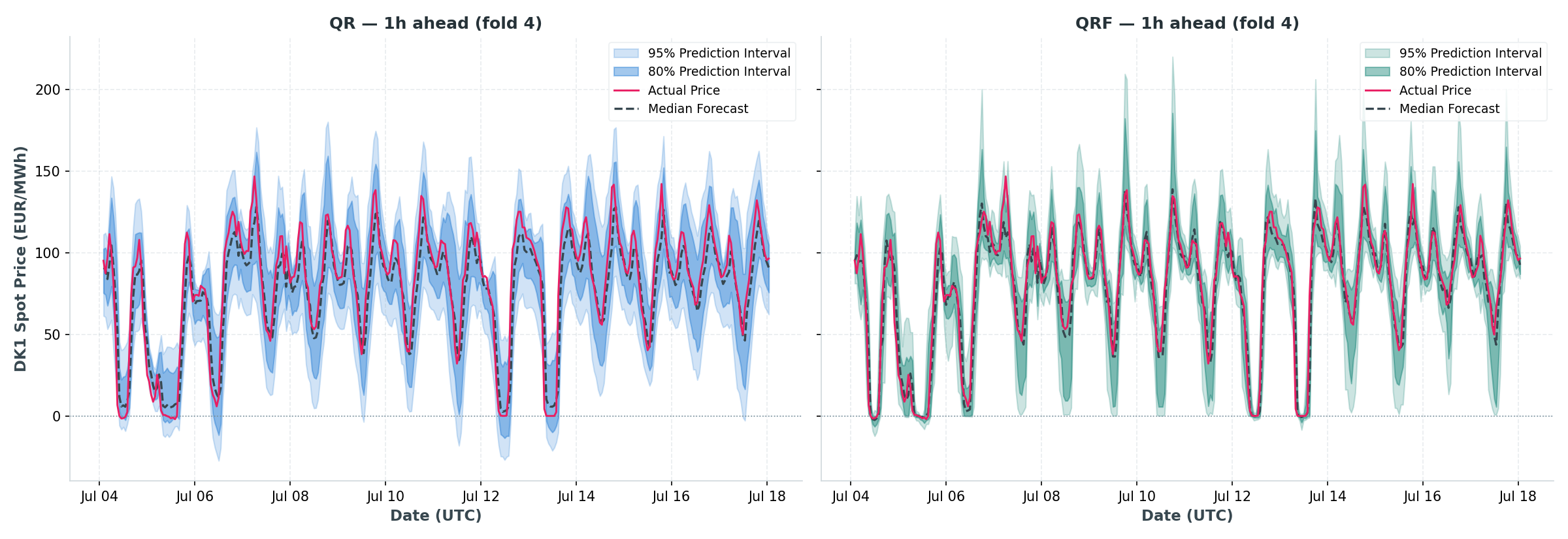 QR vs QRF, 1h-ahead, on the most recent fold’s two-week test window, with 80% and 95% prediction intervals.
Look closely at this fold (Fold 4, 4 to 18 July 2025) and QRF’s upper tail visibly sits above QR’s during the price spikes. A higher upper tail means QRF is putting more probability on extreme high prices in this specific window. That’s a good thing if those extremes actually happen, it’s better tail calibration, and a bad thing if they don’t, it’s over-dispersion and a loss of sharpness for no benefit. A few checks confirm which case this actually is:
- Exceedance count. Count how many actual prices in the fold 4 test window exceed each model’s 95th-quantile prediction; a well-calibrated 95% quantile should be exceeded roughly 5% of the time.
- One-sided upper coverage. Compute the empirical $P(y \leq \hat Q_{0.95})$ for the window and report its deviation from 0.95; a large positive deviation means the tail is too wide, a negative one means it’s too narrow.
- Interval width over time. Plot the 95% interval width for both models across the two weeks and mark the timestamps of the price spikes, to see whether QRF’s wider tail lines up with the spikes or persists everywhere.
- Rolling pinball loss at τ = 0.95. Compute a 7-day rolling pinball loss at the 0.95 quantile for both models and compare; if QRF’s rolling loss is lower around the spikes, the wider tail is earning its keep.
- PIT histogram for the fold. Build the PIT histogram restricted to fold 4 only; a histogram skewed toward 1 would confirm the upper tail is systematically too wide rather than just wide during genuine extremes.
Running the first three checks on this fold’s actual predictions:
| Model | Exceedances (τ = 0.95) | Upper coverage deviation | Mean 95% width |
|---|---|---|---|
| QR | 13 / 336 (3.9%) | +0.011 | 72.8 €/MWh |
| QRF | 4 / 336 (1.2%) | +0.038 | 54.4 €/MWh |
This is a more precise, and slightly different, story than the fan chart alone suggests. QRF’s 95% interval is narrower on average than QR’s, consistent with the pattern above, but at the single 95th quantile specifically, QRF is exceeded only 4 times out of 336 hours against a 5% nominal target, while QR is exceeded 13 times, much closer to nominal. QRF’s upper bound in this fold isn’t missing extremes, it’s overshooting them. That’s a conservative bias in this one quantile and fold, not the sharper tail its narrower average width would suggest. QR’s tail calibration is, if anything, closer to nominal here, even with a wider interval overall.
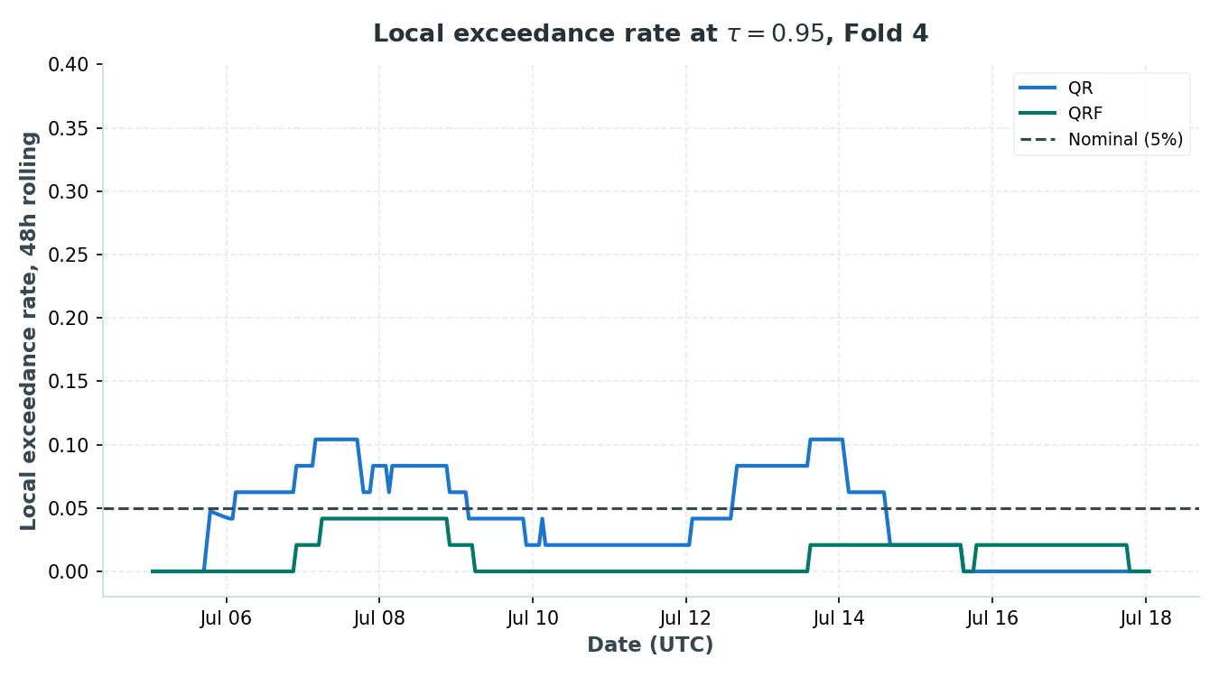 Local exceedance rates for the 95th quantile on fold 4; lower exceedance closer to 5% indicates better tail calibration.
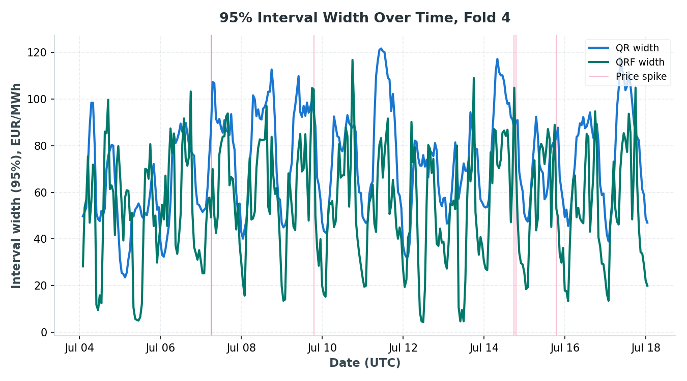 95% interval width over time for QR and QRF on fold 4; narrow and low coverage indicates under-dispersion, wide and correct coverage indicates conservative but calibrated forecasts.
3.4 Other Lead Times and Overall Calibration
That’s the full tail diagnosis for one fold at one lead time. The same walk-forward pipeline produces an equivalent fan chart for each of the other three lead times:
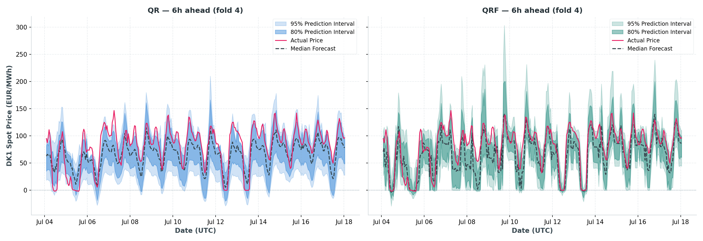 QR vs QRF, 6h-ahead.
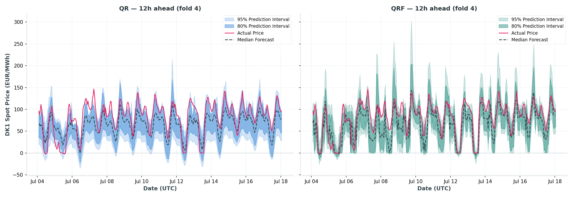 QR vs QRF, 12h-ahead.
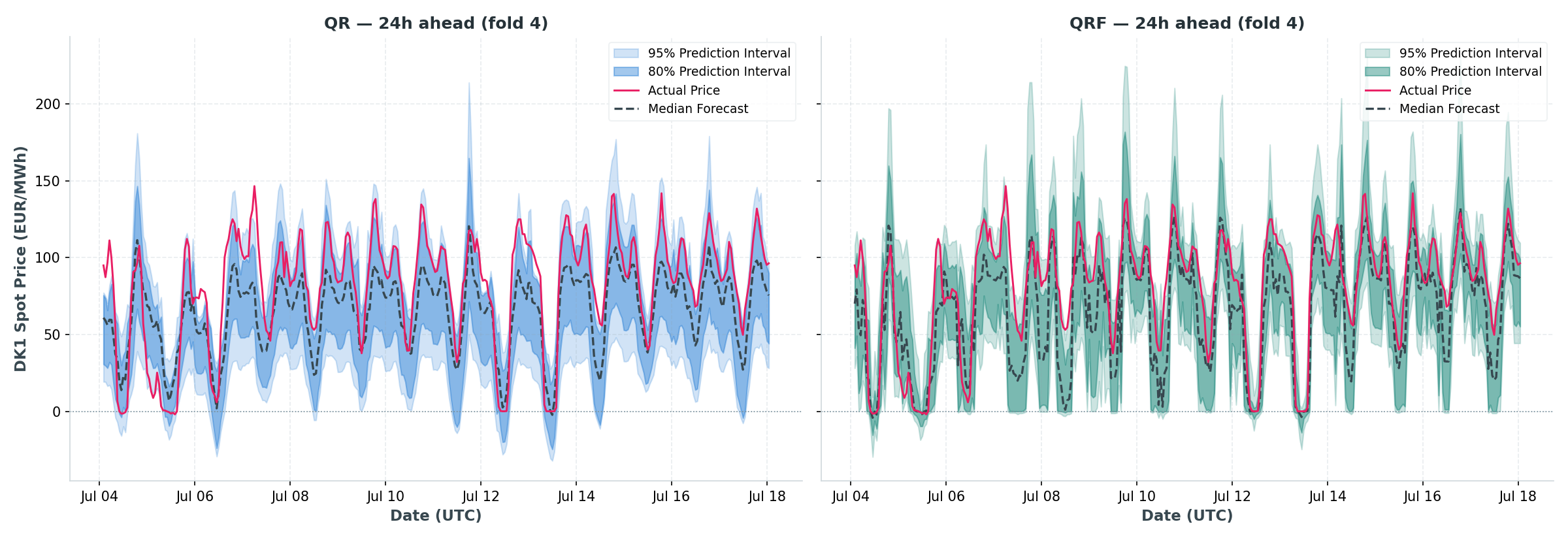 QR vs QRF, 24h-ahead.
Zooming out from any single fold to the full cross-validated picture:
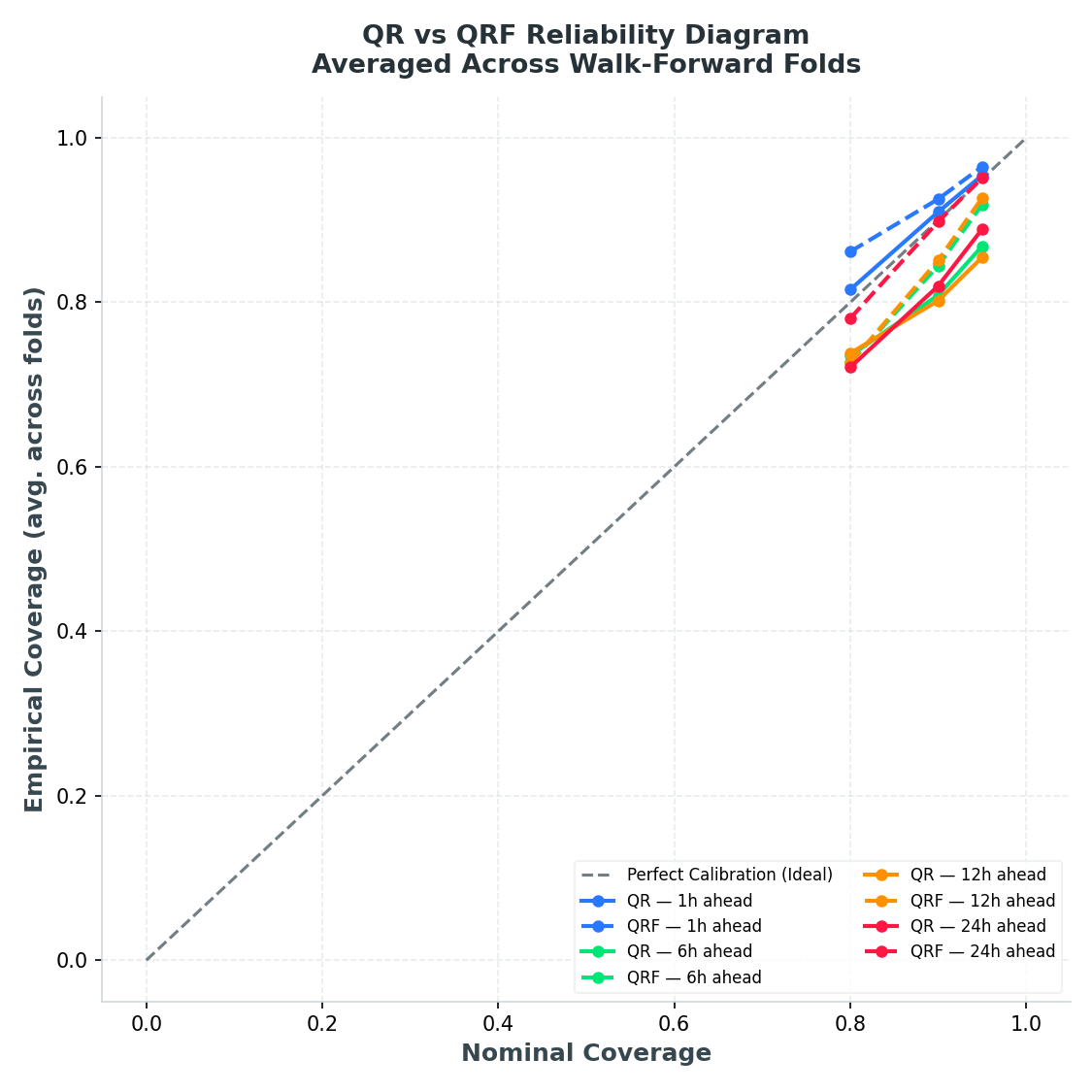 Reliability diagram (empirical vs nominal coverage) for QR and QRF, averaged across all four folds, for all four lead times.
A point sitting on the diagonal is perfectly calibrated at that nominal level. QRF’s points hug the diagonal noticeably more closely than QR’s across most lead times, the same pattern already visible in the coverage-delta table above, but compressed here into a single picture: whichever model’s markers sit closer to the dashed line, for a given colour (lead time), is the better-calibrated one at that horizon. It’s a useful sanity check on the tables rather than new information, since it’s built from the same averaged coverage numbers, just plotted instead of listed.
3.5 Likely Causes of the Calibration Collapse
- Regime mismatch. The worst-calibrated folds line up with unusual regimes: Fold 2’s test window spans Christmas and New Year, Fold 4 sits in July. Training data up to that point contains few or no comparable examples to learn from.
- Feature insufficiency. The calendar features (
dayofweek,is_weekend,is_peak) encode an ordinary working week, but say nothing about public holidays or the demand shift a holiday causes. A holiday-flag feature is the obvious next thing to try. - Model limitations. QR’s linear form has no mechanism to adapt to a regime it hasn’t been trained on. QRF’s tree splits give it more flexibility, but more flexible isn’t immune. It still degrades on regimes genuinely absent from training. Quantile crossing is one symptom specific to QR: averaged across folds it ranges from under 1% at 1h ahead to over 20% at 6h ahead in the worst fold, spiking in the same folds where coverage collapses. QRF has no such issue by construction.
All models also degrade sharply from 1h to 6h, then roughly plateau, since the lag features carry the most information about the very next hour and that advantage fades quickly once the horizon exceeds the shortest lag.
4. Conclusion
QRF is the stronger model overall, more accurate at every lead time, narrower intervals, and better calibrated for three of the four horizons, and walk-forward validation shows that conclusion holds across seasons and market regimes rather than one three-month window. QR stays competitive only at 1h ahead, where both models are already well calibrated. The real weakness isn’t either model individually: it’s calibration instability tied to regime, not just horizon, both models’ coverage collapses during holiday weeks, a failure a single train/test split would never reveal. That points to a feature problem rather than a modeling problem, so a holiday-flag feature is the most promising next step before reaching for a different algorithm.
Code
- Data.csv: the DK1 price and generation-mix data from Energi Data Service used throughout this post.
- qr_qrf_walkforward_pipeline.py: data loading, feature engineering, the QR and QRF model classes, and the walk-forward evaluation loop.
- forecasting_plots.py: every figure in this post, including the train/validate/test split diagram, the reliability diagram, the fold-4 tail diagnostics, and the calibration/sharpness quadrant plot.
- generate_fold4_diagnostics.py: reruns fold 4 only (1h ahead) to produce the exceedance-rate and interval-width-over-time figures.
- plot_calibration_sharpness_quadrant.py: the Step-4 quadrant figure, built directly from the published coverage/width numbers.
Results/folder: per-fold metrics and the cross-fold summary (mean and standard deviation per model per lead time).
Next: Part 3 compares two more approaches, bootstrapped residuals and split conformal prediction, and puts all four methods head to head.