Probabilistic Electricity Price Forecasting (Part 3)
Published:
Series: Probabilistic Electricity Price Forecasting Part: 3 (Bootstrapped Residuals)
QR and QRF, covered in Part 2, estimate the conditional distribution directly: QR fits one linear model per quantile, QRF reads every quantile off a single forest’s weighted empirical CDF. This post covers a different, older technique that instead takes a single point-forecast model and turns its residuals into an interval, adapted from skforecast’s Bootstrapped Residuals user guide and tested on real DK1 data rather than skforecast’s bike-sharing example.
Forecasting intervals with bootstrapped residuals is a method used to estimate the uncertainty in predictions by resampling past prediction errors (residuals). The goal is to generate prediction intervals that capture the variability in the forecast, giving a range of possible future values instead of just a single point estimate.
| The error of a one-step-ahead forecast is defined as the difference between the actual value and the predicted value ($e_t = y_t - \hat{y}_{t | t-1}$). By assuming that future errors will be similar to past errors, it is possible to simulate different predictions by taking samples from the collection of errors previously seen in the past (i.e., the residuals) and adding them to the predictions. |
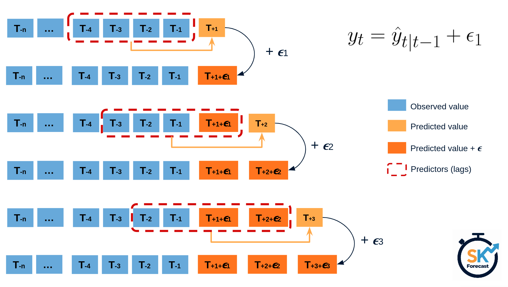 At each step, the model’s prediction is perturbed by a resampled error $\epsilon$, and that perturbed value feeds into the next step’s lags, so the errors compound forward through the recursion. Source: skforecast.org, Bootstrapped Residuals.
Repeatedly performing this process creates a collection of slightly different predictions, which represent the distribution of possible outcomes due to the expected variance in the forecasting process.
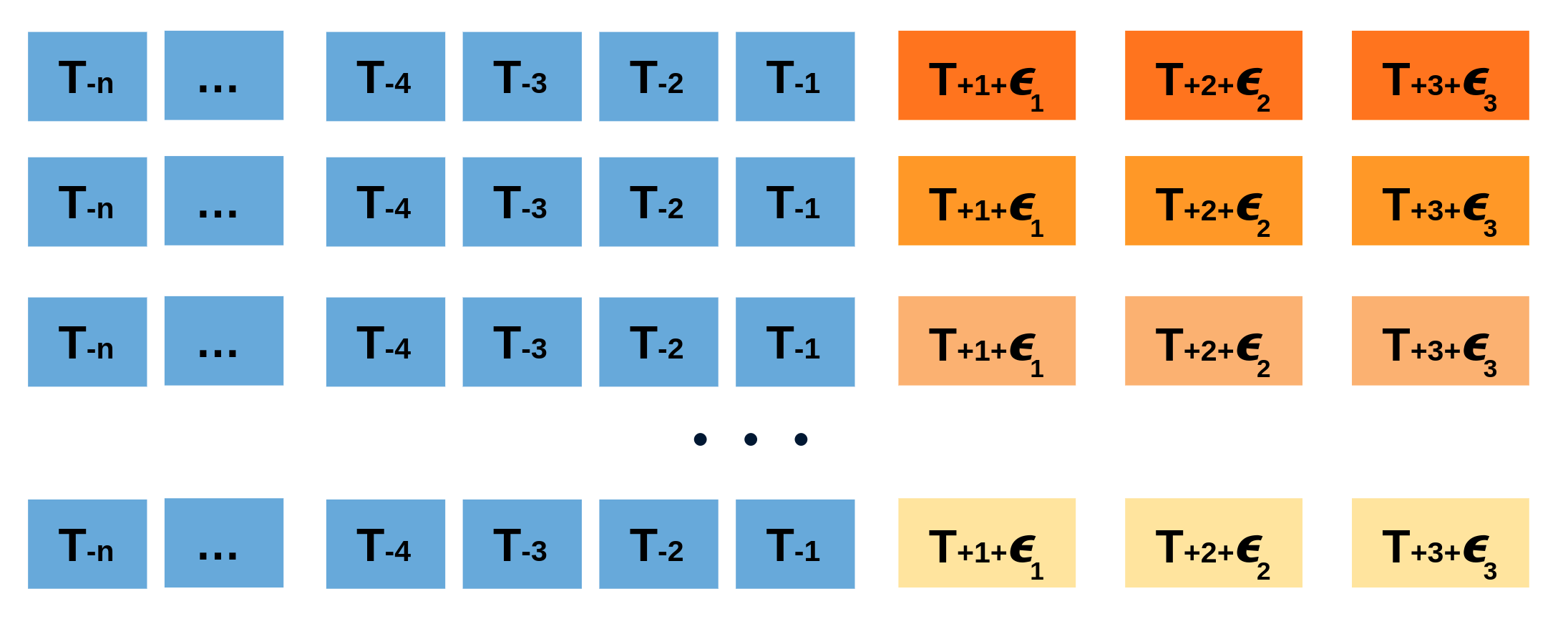 Repeated resampling of past residuals builds a collection of alternative predictions, whose spread represents forecast uncertainty. Source: skforecast.org, Bootstrapped Residuals.
Using the outcome of the bootstrapping process, prediction intervals can be computed by calculating the $\alpha/2$ and $1-\alpha/2$ percentiles at each forecasting horizon.
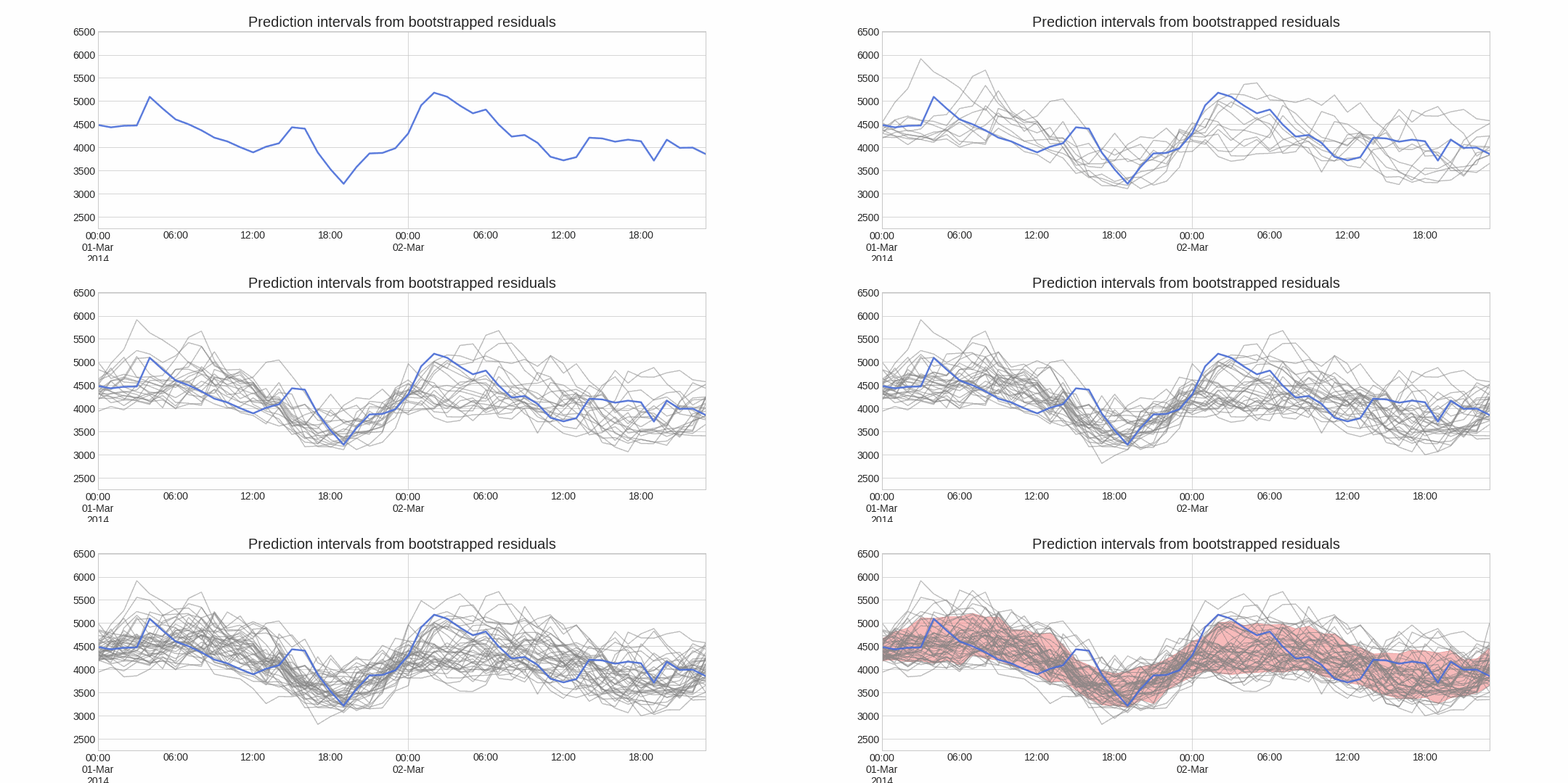 Each gray line is one bootstrap path; the band is the resulting prediction interval once percentiles are taken at each horizon. Source: skforecast.org, Bootstrapped Residuals.
Alternatively, it is also possible to fit a parametric distribution for each forecast horizon.
“One of the main advantages of this strategy is that it requires only a single model to estimate any interval. However, performing hundreds or thousands of bootstrapping iterations can be computationally expensive and may not always be feasible.” (skforecast, Bootstrapped Residuals)
Setting Up: Data and Point Model
This post reuses Part 2’s DK1 data, feature engineering, and walk-forward folds exactly (qr_qrf_walkforward_pipeline.py, included alongside this post). Rather than QR’s linear model per quantile or QRF’s forest, a single XGBoost point-forecast model stands in for the “one model” skforecast’s method is built around:
import xgboost as xgb

XGB_PARAMS = dict(n_estimators=200, max_depth=6, learning_rate=0.1, random_state=42, n_jobs=-1)
model = xgb.XGBRegressor(**XGB_PARAMS)
model.fit(X_train, y_train)
Every result below uses the same single example throughout, to keep the comparison clean: 1h-ahead, the most recent walk-forward fold (test window 4–18 July 2025), train = 12,866 rows, validation = 168 rows, test = 336 rows.
Intervals with In-Sample Residuals
By default, it’s tempting to compute residuals using in-sample data (residuals from the training set) and use those directly. However, as skforecast’s docs warn, “this can result in intervals that are too narrow (overly optimistic).”
pred_train = model.predict(X_train)
resid_train = y_train - pred_train  # in-sample: the model already fit these points

boot = rng.choice(resid_train, size=1000, replace=True)
lower = pred_test + np.quantile(boot, 0.10)
upper = pred_test + np.quantile(boot, 0.90)  # 80% interval
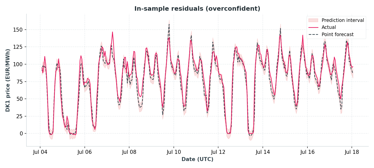 80% prediction interval built from in-sample (training-set) residuals, 1h ahead, most recent fold.
Predicted interval coverage: 52.38 %
Area of the interval: 4277.54
The interval looks tight and confident, but the coverage number gives it away: an 80% interval should catch the actual price 80% of the time, and this one manages barely half that. In-sample residuals have a standard deviation of 5.6 €/MWh; the model has already fit the training data, so its errors there systematically understate how wrong it will be on new data.
Out-of-Sample Residuals (Non-Conditioned)
To address the issue of overoptimistic intervals, it is possible to use out-of-sample residuals (residuals from a validation set not seen during training) to estimate the prediction intervals.
pred_val = model.predict(X_val)
resid_val = y_val - pred_val  # out-of-sample: validation set the model never trained on

boot = rng.choice(resid_val, size=1000, replace=True)
lower = pred_test + np.quantile(boot, 0.10)
upper = pred_test + np.quantile(boot, 0.90)
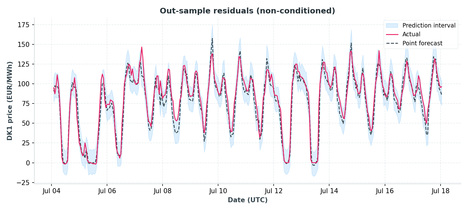 80% prediction interval built from out-of-sample (validation) residuals, same fold and horizon.
Predicted interval coverage: 89.88 %
Area of the interval: 10278.94
Out-of-sample residuals have a standard deviation of 28.6 €/MWh, five times wider than in-sample, and the resulting interval is correspondingly wider (area 10,279 vs. 4,278). Coverage jumps to 89.9%, closer to the 80% target than the in-sample version’s 52.4%, though now on the conservative side (wider than strictly needed). This is the fix skforecast’s docs recommend, and it holds here: source residuals from a split the model never trained on.
Binned Residuals (Conditioning on Predicted Value)
The bootstrapping process so far assumes that the residuals are independently distributed, so the same residual pool is used regardless of the predicted value. In reality, this is rarely true: error magnitude is often correlated with the magnitude of the prediction itself. Skforecast partitions residuals into bins associated with ranges of the predicted value, so the bootstrapping process samples from the slice of the error distribution that matches how extreme the current prediction is.
bin_edges = np.unique(np.percentile(pred_val, np.linspace(0, 100, 6)))  # 5 bins
val_bin_idx = np.digitize(pred_val, bin_edges[1:-1])
residuals_by_bin = {b: resid_val[val_bin_idx == b] for b in range(5)}
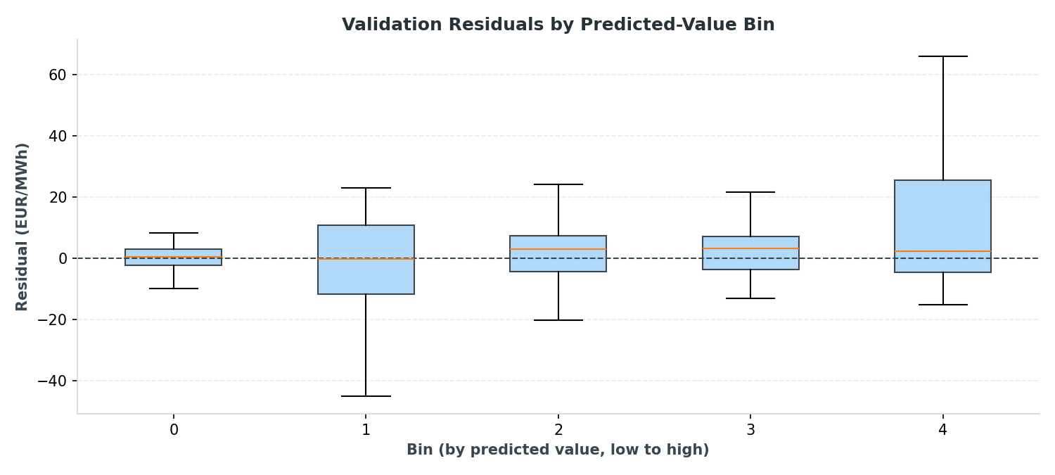 Residual spread by predicted-price bin (0 = lowest predicted prices, 4 = highest). The highest bin’s spread is visibly wider than the lowest bin’s.
The box plot confirms the assumption: bin 4 (the highest predicted prices, typically evening peak hours) has a much wider residual spread than bin 0 (the lowest predicted prices, typically overnight troughs). Bootstrapping from the matching bin, instead of the whole pool, lets the interval reflect that directly:
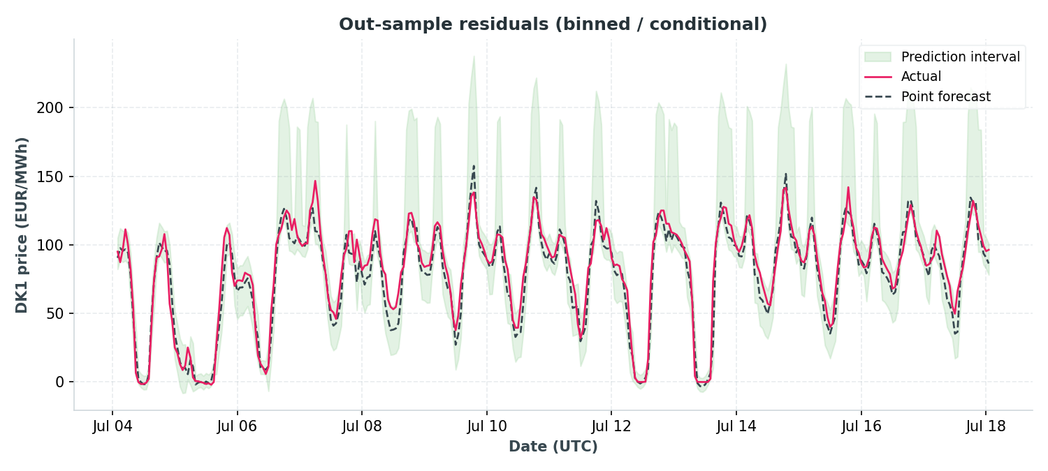 80% prediction interval built from out-of-sample residuals, binned by predicted value.
Predicted interval coverage: 85.42 %
Area of the interval: 14536.82
This is a more interesting result than a clean win. Coverage actually lands closer to the 80% nominal target than the non-conditioned version (85.4% vs. 89.9%), so calibration improved. But the total interval area went up, not down (14,537 vs. 10,279), the opposite of what binning achieved on a similar exercise applied to wave-height forecasting. Looking at the fan chart makes it clear why: the binned interval visibly narrows during calm, low-price stretches and widens sharply during price spikes, it’s reallocating width to where the uncertainty actually is, rather than shrinking everywhere. With only 168 validation rows split across 5 bins (roughly 33 rows each), the top bin’s residual pool is small enough that its bootstrap-estimated tail is noisy and, on this fold, happens to be wide. A longer calibration window would be the natural next thing to test before concluding binning helps or hurts here.
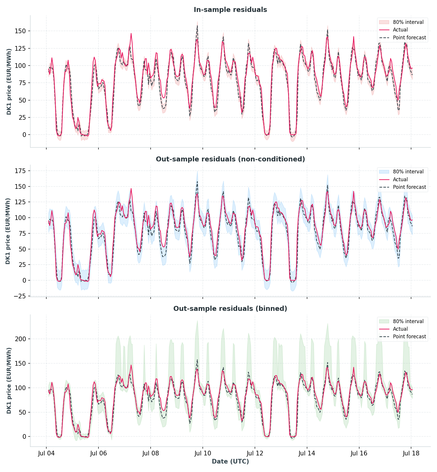 In-sample, out-of-sample non-conditioned, and binned residual intervals, same test window, stacked for direct comparison. Only the binned panel’s width visibly tracks the price level.
Prediction of Multiple Intervals
Backtesting doesn’t have to stop at one interval. The same binned-residual mechanism can produce several nominal coverage levels at once, at almost no extra cost, useful for checking calibration across the whole range rather than a single point:
for cov_pct in [10, 20, 30, 40, 50, 60, 70, 80, 90, 95]:
    alpha = (100 - cov_pct) / 100
    lo_q, hi_q = alpha / 2, 1 - alpha / 2
    # ... bootstrap from the matching bin at (lo_q, hi_q) instead of (0.10, 0.90)
| Nominal coverage | Empirical coverage |
|---|---|
| 10% | 10.7% |
| 20% | 25.3% |
| 30% | 37.2% |
| 40% | 47.0% |
| 50% | 57.7% |
| 60% | 66.7% |
| 70% | 81.2% |
| 80% | 85.1% |
| 90% | 92.9% |
| 95% | 96.4% |
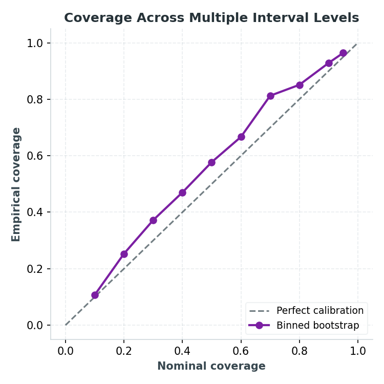 Empirical vs. nominal coverage across ten interval levels, binned method.
Every level sits at or slightly above the diagonal: a mild conservative bias (intervals a bit wider than strictly needed) rather than genuine under-coverage, consistent across the whole range rather than just the one 80% level checked earlier.
Implementation for This Project
The full implementation used to produce every result and figure in this post lives in bootstrap_residuals_deep_dive.py (included alongside this post), which reuses Part 2’s data/fold/feature code from qr_qrf_walkforward_pipeline.py directly rather than duplicating it. The core mechanism, stripped to essentials:
def bootstrap_offsets(residual_pool, quantiles, n_bootstrap, rng):
    boot = rng.choice(residual_pool, size=n_bootstrap, replace=True)
    return {q: float(np.quantile(boot, q)) for q in quantiles}

# Out-of-sample, binned by predicted value:
bin_edges = np.unique(np.percentile(pred_val, np.linspace(0, 100, n_bins + 1)))
bin_edges[0], bin_edges[-1] = -np.inf, np.inf
val_bin_idx = np.digitize(pred_val, bin_edges[1:-1])
test_bin_idx = np.digitize(pred_test, bin_edges[1:-1])

lower, upper = np.empty_like(pred_test), np.empty_like(pred_test)
for b in np.unique(test_bin_idx):
    mask = test_bin_idx == b
    pool = resid_val[val_bin_idx == b]
    offsets = bootstrap_offsets(pool, [0.10, 0.90], n_bootstrap=1000, rng=rng)
    lower[mask] = pred_test[mask] + offsets[0.10]
    upper[mask] = pred_test[mask] + offsets[0.90]
Summary
- Never calibrate on training-set residuals. In-sample residuals here understated the true error spread by roughly 5x (5.6 vs. 28.6 €/MWh) and delivered 52% actual coverage against an 80% claim, badly overconfident, and this is a real, measured failure mode on this data, not a hypothetical one.
- Out-of-sample (validation) residuals fix the coverage problem, at the cost of a much wider interval. On this fold, 89.9% actual coverage against an 80% nominal target, closer than in-sample but now on the conservative side.
- Binning by predicted value redistributes width rather than shrinking it uniformly. Coverage improved (closer to nominal) but total area increased, because the highest-price bin genuinely carries more uncertainty and the interval now reflects that honestly, at the cost of a noisier bootstrap in the smallest bins with only ~33 validation rows each.
- Coverage should be checked across the whole range of interval levels, not just one. The multi-level sweep here showed a mild conservative bias throughout (10%–95%), rather than a single level’s number telling the whole story.
References
- Skforecast. Probabilistic Forecasting: Bootstrapped Residuals. skforecast.org/0.15.0/user_guides/probabilistic-forecasting-bootstrapped-residuals
Code
- Data.csv: the same DK1 data used in Part 2.
- qr_qrf_walkforward_pipeline.py: shared data loading, feature engineering, and fold generation (same file as Part 2, included here so this post runs standalone).
- bootstrap_residuals_deep_dive.py: in-sample vs out-of-sample vs binned residual comparison, and the multiple-intervals sweep.
- bootstrap_deepdive_plots.py: every figure in this post.
Results/DeepDive/folder: method comparison and multiple-intervals coverage.
Next: Part 4 will cover split conformal prediction and put it head to head against bootstrapped residuals, QR, and QRF.