Operational LLM AI-Agent for Energy Community BESS Management
Published:
This post answers Question 2 of the written assessment for a PhD candidate interview at Mälardalen University: "PhD Candidate Interview Questions: AI-Agent Development for Energy Systems". The 1-page architecture summary submitted for Part A is available for reference; this post is the write-up of Part B, the implementation prototype.
1. Why an Agent Instead of a Stand-Alone Optimiser
A Battery energy storage system (BESS) in a small energy community must balance three misaligned signals:
- Evening-peaking demand
- Midday-peaking solar generation
- Spot electricity price varies in the renewable electricity market nowadays
A mathematical optimiser can schedule the BESS using forecasts of these variables. However, what it cannot do is explain its reasoning, justify its decisions, or address operator questions when the resulting plan appears unexpected. For example, charging battery when the prices are not low. Because the optimizer expects a future high‑demand period and needs sufficient state‑of‑charge.
That’s the gap an LLM agent is meant to fill: not replacing the optimizer, but sitting on top of it, translating “should we discharge in the next two hours” into a tool call, and translating the tool’s numeric output back into a sentence a non-specialist can act on. This post walks through a small end-to-end system built around that idea, from synthetic load and PV data through a day-ahead price forecaster, a Pyomo battery scheduler, and a provider-agnostic ReAct agent with three tools.
2. Main Pipeline
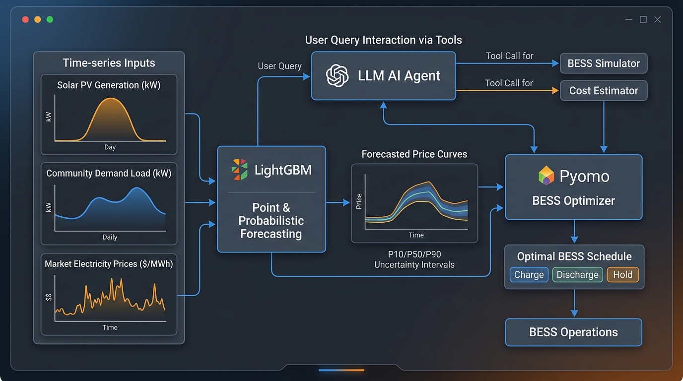
Above is the Graphical abstract for the main pipeline. First, three time series data (solar PV generation, community demand, and market price) feed LightGBM, which does both point and probabilistic forecasting (Boostrapped Bin Residual). LightGBM’s price forecast comes out as a P10/P50/P90 band; its load and PV forecasts feed forward too. Both go into the Pyomo BESS optimizer, which solves the Linear Program (LP) and produces the optimal schedule (charge, discharge, or hold), which then drives the actual BESS operations.
The LLM agent sits to one side of that pipeline, not inside it. A user query goes to the agent, which issues tool calls (BESS Simulator, Cost Estimator, in the diagram, mapping to bess_simulator and electricity_cost_estimator in the code) rather than answering from its own reasoning. Those tools read the optimizer’s already-solved schedule, and their output flows back up into the agent so it can answer in plain language, grounded in whatever Pyomo actually decided rather than a guess.
2.1 Data
Load and PV are synthetic, generated to look like a real energy community rather than pulled from a live meter. The one real dataset in the pipeline is the day-ahead spot price for the DK1 bidding zone: hourly, sourced from Denmark’s Energi Data Service, 2024-01-01 through 2025-09-30 (15,336 hours).
Load. The community load is the sum of five sectors, each built from the same shape and hit with independent Gaussian noise:
\[P_{\text{load}}(t) = \big(P_{\text{base}} + P_{\text{diurnal}}(t)\big) \times M_{\text{day}}(t) + \epsilon(t)\]A constant standby load plus a time-of-day shape, scaled down on weekends by $M_{\text{day}}(t)$, plus Gaussian noise $\epsilon(t)$. Each sector below just plugs its own base level, diurnal shape, and weekend multiplier into this same template.
| Sector | Base (kW) | Peak addition (kW) | Active window | Weekend multiplier |
|---|---|---|---|---|
| Office | 10 | 80 (dual peak, 10:00 & 15:00) | 08-18 weekdays | 0.1 |
| Logistics | 20 | +120 in the morning / +150 in the afternoon | 06-09 & 17-20, Mon-Sat | 0.15 (Sun) |
| Manufacturing | 80 | 220 (shifts 1-2) / 120 (night shift) | 3 shifts, weekdays | 0.15 |
| EV (passenger) | 0 | 200 | 08:00-13:00 weekdays (unmanaged charging) | 0 |
| EV (HGV) | 0 | 600 | 18:00-23:00 weekdays (depot charging) | 0 |
Total load is the sum of all five, clipped at zero; over the full series it peaks at 933 kW. Full per-sector equations (including the dual-Gaussian office curve and the shift step function) are in Load_Logic.md.
PV. ERA5 gives Surface Solar Radiation Downwards (SSRD, J/m²) per hour, converted to irradiance and scaled to a 50 MWp plant:
\[G_{\text{avg}} = \frac{\text{SSRD}}{3600}\ \left[\text{W/m}^2\right], \qquad P_{\text{PV}}(t)\ [\text{kW}] = G_{\text{avg}} \times A_{\text{total}}\,\eta_{\text{PV}}\,\eta_{\text{system}}\,\eta_{\text{temp}} = G_{\text{avg}} \times 42.75\]SSRD is the energy that landed on each square meter over the hour (joules); dividing by the 3,600 seconds in an hour converts that to an average power density. Multiplying by the panel area and the three efficiency factors converts irradiance into plant output; since the area and efficiencies are fixed for this plant, they collapse into the single constant 42.75.
| Parameter | Value |
|---|---|
| Plant capacity | 50 MWp (100,000 x 500 Wp panels) |
| Active panel area,$A_{\text{total}}$ | 250,000 m² |
| Module efficiency,$\eta_{\text{PV}}$ | 20% |
| System losses (inverter, cabling, soiling) | 10% |
| Nordic temperature derating | 5% |
| Combined scaling factor | 42.75 |
At clear-sky peak (1000 W/m²) that’s 42.75 MW; full derivation, plus a sample irradiance-to-output table, is in PV_50MW_Scaling_Logic.md.
2.2 Forecasting the price
LightGBM replaces the quantile regression forest used in an earlier post in this series, mainly for speed at this data volume. Rather than one recursive model, each lead time gets its own model, trained directly on the target $k$ hours ahead:
\[\hat{P}(t+k) = f_k(X_t), \quad k \in \{1, \dots, 24\}\]A separate model $f_k$ for each horizon, so the price 24 hours out is predicted directly from today’s features $X_t$, not by chaining 24 one-hour-ahead predictions into each other and compounding their errors.
| Feature group | Variables |
|---|---|
| Calendar | hour, day of week, month, weekend flag |
| Autoregressive | price lags:$t-k$, $t-k-24$, $t-168$; 24h rolling mean |
Uncertainty comes from a binned residual bootstrap instead of a second set of quantile models: out-of-fold validation residuals are grouped into 15 bins by predicted price level, and a test prediction draws its P10/P90 offsets from the matching bin (5,000 bootstrap samples), so calm-period bands stay narrow and volatile-period bands stay wide:
\[\hat{P}_{\text{P10}}(t+k) = \hat{P}_{\text{test}}(t+k) + q_{10}, \qquad \hat{P}_{\text{P90}}(t+k) = \hat{P}_{\text{test}}(t+k) + q_{90}\]$q_{10}$ and $q_{90}$ are the 10th and 90th percentile of the residuals bootstrapped from the matching bin; adding them to the point forecast shifts it down and up to bound the interval around that point, without needing a separate model trained for each quantile.
Full pipeline detail (the 15-bin edges, monotonicity correction) is in Forecasting_Logic.md.
2.3 Sizing the battery
Before scheduling day to day, the battery needs a capacity. bess_sizing.py solves a Pyomo linear program, GLPK backend, once per candidate capacity, over the full 2024-01-01 to 2025-06-06 historical window:
Three terms summed over the horizon: money spent importing at the buy price, a penalty proportional to how much the battery gets cycled (so it doesn’t charge and discharge for a fraction of a cent of arbitrage margin), minus revenue earned exporting at the sell price. The solver picks the hour-by-hour charge/discharge schedule that minimizes this net cost, subject to the power balance, the grid import/export cap, and the state-of-charge dynamics:
\[E(t) = E(t-1) + \Big(P_{\text{ch}}(t)\,\eta_{\text{ch}} - \frac{P_{\text{dis}}(t)}{\eta_{\text{dis}}}\Big)\]Next hour’s stored energy is this hour’s energy, plus what got charged in after charging losses, minus what got discharged out grossed up for discharging losses. That asymmetry ($\eta_{\text{ch}}$ multiplies, $\eta_{\text{dis}}$ divides) is what makes round-trip efficiency below 100%: charging 100 kWh in stores less than 100 kWh, and getting 100 kWh back out costs more than 100 kWh of stored energy.
| Parameter | Value |
|---|---|
| Candidate capacities tested | 250, 500, 1000, 1500, 2000 kWh |
| Inverter power | 0.5C (e.g. 750 kW at 1500 kWh) |
| SoC bounds | 15-95% |
| Round-trip efficiency$\eta_{\text{ch}}\eta_{\text{dis}}$ | 90.25% (0.95 each way) |
| Degradation penalty$C_{\text{deg}}$ | 0.40 DKK/kWh throughput |
| Grid import/export cap | 500 kW |
The two smallest capacities came back infeasible: not enough discharge power to keep peak import under the 500 kW grid limit. Of the feasible sizes, 1500 kWh / 750 kW led on net annual benefit:
| Capacity (kWh) | Power (kW) | CAPEX (DKK) | Annual OPEX (DKK) | Annual savings (DKK) | Payback (years) |
|---|---|---|---|---|---|
| 1500 | 750 | 2,797,500 | 41,962.50 | 239,508.59 | 11.68 |
| 2000 | 1000 | 3,730,000 | 55,950.00 | 307,858.74 | 12.12 |
Eleven and a half years, under a conservative 10-year straight-line amortization, is the honest number for pure spot-price arbitrage plus self-consumption. It moves with the financing assumptions actually used in industrial storage projects:
| Adjustment | Effect on the 1500 kWh case |
|---|---|
| 15-year amortization (realistic cycle life vs. 10-year straight-line) | Net annual benefit turns positive: +11,046 DKK/year |
| 40% CAPEX subsidy (common for EU storage/grid projects) | Payback drops to about 7.0 years |
| Registering for Nordic ancillary markets (FCR-D, FFR) on top of arbitrage | Revenue roughly doubles/triples; payback to about 4-6 years |
None of these are modeled in the LP itself, they’re back-of-envelope sensitivity from BESS_Optimization_and_Forecast_Logic.md, not a re-solve.
2.4 Scheduling the week
With the size fixed, daily_optimization.py solves a second Pyomo/GLPK model, a one-shot 168-hour LP over a rolling 7-day window, using the LightGBM price forecast (with its P10/P90 band) instead of historical actuals:
| Metric (2025-06-07 to 2025-06-13) | Value |
|---|---|
| Savings vs. no-BESS baseline | 2,064.49 DKK |
| Grid import peak | 500 kW |
| Grid export peak | 500 kW |
| Total battery charging | 2,268.15 kWh |
| Total battery discharging | 2,545.75 kWh |
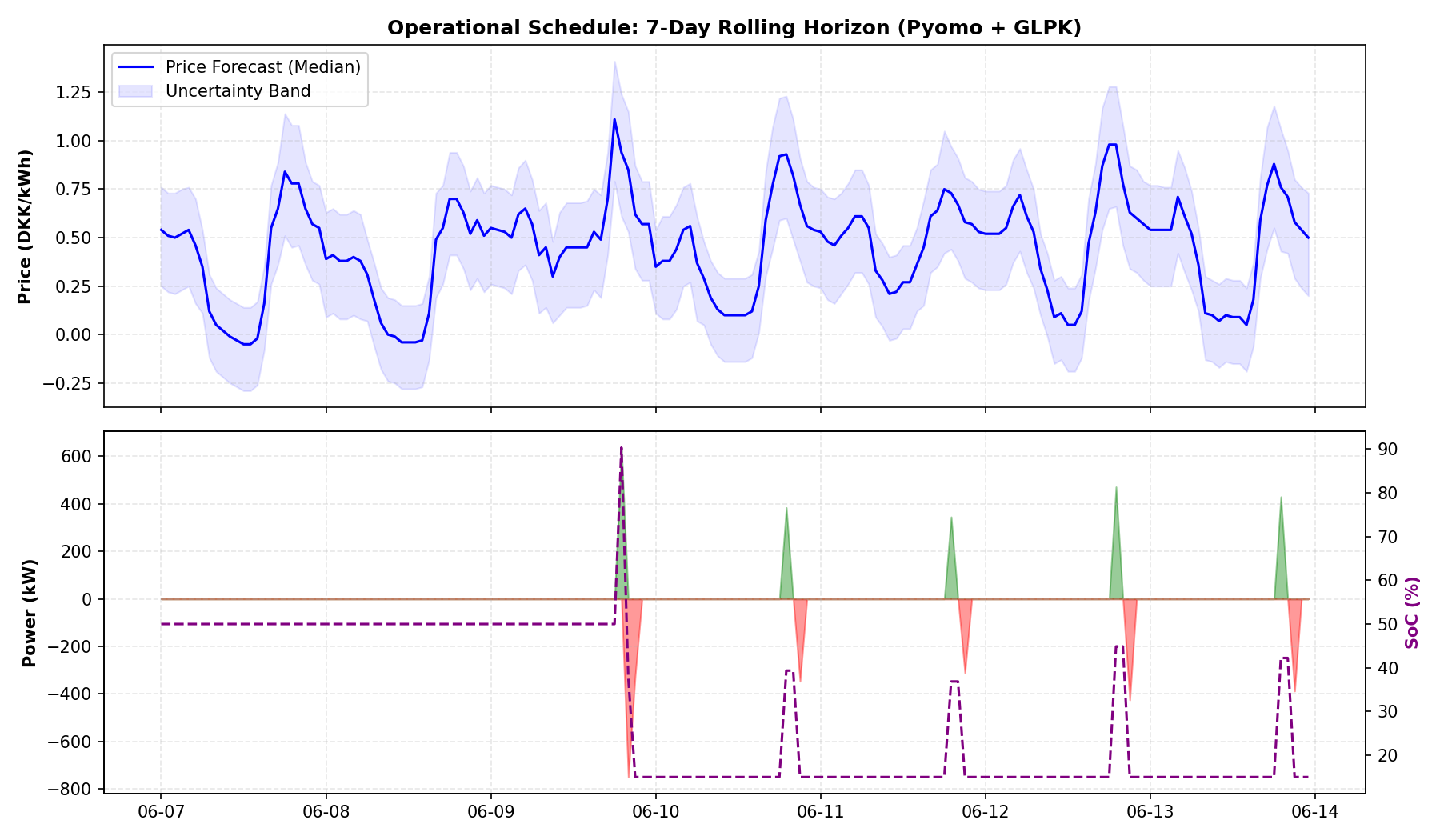 7-day dispatch schedule: spot price with its P10-P90 band on top, battery charge/discharge and state of charge below.
The script also writes a zoomable interactive HTML version with Plotly, useful for looking at any individual day up close rather than squinting at a week compressed into one static plot.
3. Agent Architecture and Integration
The scheduler produces a schedule, not an answer; the agent’s role is to mediate between the two.
3.1 Response Latency Handling
Advisory queries, such as asking whether to discharge now, are answered in seconds by reading the already-solved schedule; nothing gets recomputed on the request. A query that needs a fresh solve, a large forecast revision or a genuine what-if scenario, triggers an asynchronous optimization run instead: the agent replies immediately with the last valid schedule and a staleness note, or reports that it is recomputing, rather than making the user wait on the solver. The optimizer runs on its own hourly cadence, independent of the chat interface, which never blocks on a solver call.
3.2 Tool Definitions
All three tools read from the same solved schedule CSV, keeping their outputs consistent and traceable to a single optimizer run. The LLM never computes these figures itself: it emits a JSON tool call, Python executes it deterministically, and the model’s role is limited to narrating the returned values.
bess_simulator: validates a proposed charge/discharge action against the 15-95% SoC bounds; flags a violation rather than silently clamping it.self_consumption_calculator: sums PV generation and load over a time window; reports the fraction of local solar consumed on site versus exported.electricity_cost_estimator: computes net grid cost (DKK) over a window, with ano_bessmode for baseline comparison.
3.3 Multi-Provider Model Support
bess_agent.py is framework-independent, with no LangChain, LlamaIndex, or other orchestration dependency in between. Provider selection runs off whichever API key is present in the environment, across OpenAI, Anthropic, Gemini, DeepSeek, or a local Ollama model, plus a key-free mock mode for offline testing. Every provider is held to the same response contract: any price figure must be stated as an explicit uncertainty range (P10-P90) with the schedule source cited, and a bare point number counts as an incomplete answer.
Two required queries exercise the loop end to end:
- “Should we charge or discharge the battery in the next two hours given the current conditions?” → calls
bess_simulator; response: “Recommend discharging at 750 kW, moving SoC from 50% to 15%. Price is forecast at about 0.4 DKK/kWh, range 0.1-0.64 DKK/kWh (P10-P90). (Per the day-ahead LP solve.)” - “What was our self-consumption rate yesterday and how could it be improved?” → calls
self_consumption_calculator; reports the rate, recommends shifting charging into the midday PV surplus, and cites the schedule source.
4. Interactive Demonstration
GitHub Pages is static hosting, so no server is available to run a live model. The embed below is a client-side JavaScript port of the three tools above, running against the same solved 7-day schedule; the tool math and response figures are identical to bess_agent.py, not a simplified mock. The one shortcut is query routing: it’s regex-based rather than an LLM call, and recognizes only the three query shapes covered in Section 3.3.
If the embed doesn’t load, open the demo directly.
5. Limitations and Future Work
The load and PV forecast error used in the scheduler is synthetic Gaussian noise (5% load, 12% PV), not the output of a trained forecaster; the price forecast is the only component validated end to end against real held-out data. The dispatch model is also a single 7-day solve rather than a rolling re-optimization that updates as new forecasts arrive, and EV and heavy-goods-vehicle charging flexibility isn’t yet modeled as shiftable load within the LP.
6. Code
01_Load/generate_load_profiles.py— synthesizes the community load profile (double-Gaussian diurnal peaks, weekday/weekend logistic modulation).02_PV_Generation/simulate_pv_generation.py— scales ERA5 irradiance to a 50 MW solar farm.05_Optimisation_and_Forecast/bess_sizing.py— Pyomo/GLPK capacity sizing sweep and financial feasibility report.05_Optimisation_and_Forecast/daily_optimization.py— LightGBM price forecast plus binned residual bootstrap, 7-day Pyomo/GLPK dispatch schedule, static and interactive plots.06_LLM/bess_agent.py— the ReAct tool-use agent loop and its three tools, with the multi-provider router.06_LLM/bess_agent_demo.html— the client-side demo above: the same three tools ported to JavaScript, with a regex router standing in for the LLM.
The full project, including the synthetic data, the GLPK solver package, and every intermediate result file, lives in this folder on GitHub. GitHub’s own directory download button there gets you a zip of everything at once, so it isn’t duplicated as a separate download on this page.