
Icing formation in Wind turbines in Cold climate region (part 2) - IEA Task 19
❄️ IEA Wind Task 19 — Ice Loss Method
A standardized, open-source pipeline to detect, classify, and quantify wind turbine production losses due to rotor icing — using only standard SCADA data.
Table of Contents
- Background & Motivation
- Method Overview
- Input Data
- Step 1: Reference Power Curve
- Step 2: Icing Event Classification
- Step 3: Production Loss Quantification
- Outputs
- Installation & Usage
- Example Results (ExampleDataset, 2003)
- Limitations
- Further Development
- References
1. Background & Motivation
Wind turbines operating in cold climates — Scandinavia, Canada, Central Europe — deal with a persistent problem: ice accretes on the rotor blades, disrupts the aerodynamic profile, and silently erodes power output. In the worst case, turbines shut down completely. In an unexpected scenario, an iced nacelle anemometer reports an artificially low wind speed, causing the turbine to overestimate its own performance.
The economic impact is real. What makes it difficult is that the industry has historically had no agreed-upon way to measure it. Common approaches include:
- Applying a fixed -15% or -25% drop from the nominal power curve as an icing indicator.
- Using multiples of the standard deviation from mean power as a detection threshold.
Neither approach is grounded in physics, and both produce inconsistent results across sites and turbine models. You cannot compare icing losses between two wind farms if each used a different method.
IEA Wind Task 19 is an international expert group formed to solve exactly this. Their Ice Loss Method defines a single, reproducible algorithm — based on percentile statistics and temperature thresholds — that anyone with standard SCADA data can apply. No icing sensors required. No site-specific assumptions hard-coded in.
The open-source Python implementation is available at: 👉 https://github.com/IEAWind-Task19/IceLossMethod
2. Method Overview
The method works in three sequential steps:
SCADA Time Series (10-min resolution)
         │
         ▼
┌─────────────────────────────────────┐
│  Step 1: Build Reference Power Curve │  ← warm-weather, clean data only
│  → P10, P50 (median), P90 per bin   │
└──────────────────┬──────────────────┘
                   │
                   ▼
┌─────────────────────────────────────┐
│  Step 2: Detect Icing Events        │  ← compare full time series to reference
│  → IEa (reduced power)             │
│  → IEb (shutdown)                  │
│  → IEc (overproduction)            │
└──────────────────┬──────────────────┘
                   │
                   ▼
┌─────────────────────────────────────┐
│  Step 3: Quantify Production Losses │  ← IEa + IEb only
│  → ΔP(t), E_ice [kWh], L_ice [%]  │
└─────────────────────────────────────┘
The method is robust by design: it uses percentile-based statistics rather than mean/standard deviation, makes no assumption about normal data distribution, and requires three consecutive 10-minute periods (30 min) to confirm an icing event — minimising false alarms from short wind gusts or transient faults.
3. Input Data
The code processes one turbine at a time. For a multi-turbine site, a separate configuration file is needed per turbine.
3.1 Minimum Required Signals
| Column | Signal | Unit | |
|---|---|---|---|
| Index | Column | Signal | Unit |
| 0 | Timestamp | UTC timestamp (10-min intervals) | — |
| 1 | Wind speed [m/s] | Nacelle anemometer wind speed | m/s |
| 2 | Wind direction [deg] | Wind direction | deg |
| 3 | Ambient temperature [C] | Nacelle or mast temperature | °C |
| 4 | output power [kW] | Turbine electrical output | kW |
| 5 | State | Operational state (OK = normal) | — |
| 6 | Status | Stop/fault indicator (STOP = stopped) | — |
| 7 | Ice detected | Ice detector signal (WHAT = ice alarm) | — |
| 8 | IPS | Blade heating status (ON/OFF) | — |
3.2 Example Dataset Format (2003 — ExampleDataset)
This repository is demonstrated using the ExampleDataset — a synthetic one-year SCADA time series at 10-minute resolution covering the full year 2003. The dataset has the following structure:
Timestamp,Wind speed [m/s],Wind direction [deg],Ambient temperature [C],output power [kW],Status,State,Ice detected,IPS
1.1.2003 0:00,9.7,42.1,-15.7,1387,OK,OK,NO,OFF
1.1.2003 0:10,9.3,44.9,-15.6,990,OK,OK,NO,OFF
...
Key properties of this dataset:
- Period: 1 January 2003 — 31 December 2003
- Resolution: 10 minutes (52,560 records in a complete year)
- Turbine model: 2 MW rated capacity (
rated power = 2000kW) - Site elevation: 100 m above sea level (used for air density correction)
- Temperature range: sub-zero winters present → icing events expected
- State codes:
OK= normal production,STOP= turbine stopped - Ice detection: column present (
WHAT= ice alarm triggered) - IPS: column present but
heating = False— no active blade heating at this site
This dataset is included in the official IEA Task 19 repository and is freely available for testing and validation purposes.
4. Step 1: Reference Power Curve
The reference power curve is the cornerstone of the method. Every icing event is detected by comparing the full time series against this baseline. The baseline must represent the turbine’s clean, ice-free aerodynamic performance — so the data used to build it is filtered strictly.
4.1 Filtering for Clean Reference Data
Only data meeting all of the following criteria is used:
temperature > +3°C          → ice-free condition (safe margin above 0°C)
turbine state == normal      → full production, no faults or maintenance
output power > 1% of P_rated → exclude near-zero "spinning but not generating" records
The temperature threshold of +3°C is set deliberately above 0°C. At temperatures just below 0°C, icing influence on the rotor is already possible; setting the threshold at +3°C provides a conservative margin. This logic corresponds directly to the temperature_filter_data() function in the code:
# From t19_counter.py — reference data construction
s_reference_data = aepc.state_filter_data(temperature_corrected_data)   # state filter
d_reference_data = aepc.temperature_filter_data(s_reference_data)        # temp > +3°C
reference_data   = aepc.power_level_filter(d_reference_data)             # power > threshold
4.2 Air Density Correction
Before binning, wind speed is corrected for air density using the ISO 2533 standard atmosphere model. Cold, dense air produces more power at a given wind speed than warm air. Without this correction, winter data would appear to overperform relative to summer data, introducing a systematic bias into the reference.
temperature_corrected_data = aepc.air_density_correction(data)
4.3 Binning by Wind Speed
The clean reference data is binned by wind speed. Each bin collects all records within a given wind speed range and computes the following statistics:
| Statistic | Symbol | Role |
|---|---|---|
| Median power | $P_{50}(v_\text{bin})$ | Reference power for loss calculation |
| 10th percentile | $P_{10}(v_\text{bin})$ | Lower detection threshold (IEa, IEb) |
| 90th percentile | $P_{90}(v_\text{bin})$ | Upper detection threshold (IEc) |
| Standard deviation | $\sigma(v_\text{bin})$ | Power curve uncertainty |
| Sample count | $n(v_\text{bin})$ | Data density check |
Default binning parameters (configurable in the .ini file):
[Binning]
minimum wind speed    = 0      ; m/s
maximum wind speed    = 20     ; m/s
wind speed bin size   = 1      ; m/s (default)
wind direction bin size = 360  ; single direction bin by default
A minimum of 6 hours of data per bin is recommended for a statistically representative result. Bins with too few samples are interpolated linearly from adjacent bins to avoid gaps in the reference curve.
5. Step 2: Icing Event Classification
With the reference thresholds computed, the full dataset (all temperatures, all operational states) is scanned chronologically to detect icing events. Three distinct classes are defined.
📷 [Insert figure: Icing class diagram showing IEa (reduced production zone), IEb (shutdown zone), IEc (overproduction zone) relative to the power curve and P10/P90 bounds]
Class IEa — Reduced Power Output
Ice accretes on the blade surface and gradually degrades aerodynamic lift. The turbine remains running, but power output drops below what the wind speed should produce.
Start condition — all of the following must hold for ≥ 30 consecutive minutes:
\[T_\text{amb} < 0°\text{C}\] \[P < P_{10}(v_\text{bin})\]→ Icing event class (a) starts.
End condition — the following must hold for ≥ 30 consecutive minutes:
\[P > P_{10}(v_\text{bin})\]→ Icing event class (a) ends.
Recorded in output as: Production losses due to icing
Class IEb — Icing-Induced Shutdown
In severe cases, the turbine safety system triggers a full stop — typically due to rotor imbalance, excess tower vibration, or ice-induced fault codes. Unlike IEa where the turbine stays running at reduced output, IEb captures the standstill periods.
Start condition — all of the following must hold:
\[T_\text{amb} < 0°\text{C}\] \[P < P_{10}(v_\text{bin}) \quad \text{for 10 consecutive minutes}\] \[P < 0.5\% \cdot P_\text{rated} \quad \text{for 20 consecutive minutes}\]→ Standstill due to icing class (b) starts.
End condition — the following must hold for ≥ 30 consecutive minutes:
\[P > P_{10}(v_\text{bin})\]→ Icing event class (b) ends.
Recorded in output as: Standstill due to icing
Note on manual review: Some turbines shut down due to icing before the power even crosses the $P_{10}$ threshold — particularly turbine models that are sensitive to rotor imbalance. The algorithm may miss these. Manual inspection of wintertime fault codes (e.g., excess side-to-side tower vibration, nacelle wind speed inconsistency) is recommended to supplement the automatic detection, as standstill losses are typically larger than operational losses.
Class IEc — Iced Anemometer / Overproduction
When ice accretes on the heated nacelle anemometer, it reports an artificially low wind speed. The turbine controller, perceiving weaker wind than reality, does not pitch back the blades — resulting in power output that exceeds the reference curve prediction. This is a measurement artifact.
Start condition — all of the following must hold for ≥ 30 consecutive minutes:
\[T_\text{amb} < 0°\text{C}\] \[P > P_{90}(v_\text{bin})\]→ Iced anemometer overproduction event class (c) starts.
End condition — the following must hold for ≥ 30 consecutive minutes:
\[P < P_{90}(v_\text{bin})\]→ Icing event class (c) ends.
Recorded in output as: Iced anemometer overproduction
Summary of the Three Classes
| Class | Name | Temperature | Power Condition | Duration Threshold | Quantified? |
|---|---|---|---|---|---|
| IEa | Reduced production | $T < 0°C$ | $P < P_{10}$ | ≥ 30 min | kWh + % |
| IEb | Icing shutdown | $T < 0°C$ | $P < P_{10}$ then $P \approx 0$ | 10 min + 20 min | kWh + % |
| IEc | Overproduction | $T < 0°C$ | $P > P_{90}$ | ≥ 30 min | Duration only |
6. Step 3: Production Loss Quantification
Production losses are evaluated exclusively for IEa and IEb events.
For each 10-minute time step $t$ within an IEa or IEb event, the instantaneous power deficit is defined as:
\[\Delta P(t) = P_{\mathrm{ref}}\big(v_{\mathrm{bin}}(t)\big) - P_{\mathrm{meas}}(t) \tag{1}\]where:
- $P_{\mathrm{ref}}$ is the median ($P_{50}$) reference power corresponding to the wind speed bin at time $t$,
- $P_{\mathrm{meas}}(t)$ is the SCADA-measured power output.
The cumulative energy loss over an icing period $[t_0, t_n]$ is:
\[E_{\mathrm{ice}} = \sum_{t=t_0}^{t_n} \Delta P(t)\,\Delta t \tag{2}\]where:
- $\Delta t = \frac{1}{6}$ h (10-minute SCADA resolution).
The relative production loss is expressed as a percentage of the expected reference production:
\[L_{\mathrm{ice}}(\%) = \frac{E_{\mathrm{ice}}}{E_{\mathrm{ref}}} \times 100 \tag{3}\]where:
- $E_{\mathrm{ref}}$ is the total expected energy based on the reference power curve over the same period.
IEc is not energy-quantified. When the anemometer is iced, the measured wind speed is unreliable — there is no valid reference power to compare against. Only the total duration in hours of IEc events is reported. If IEc hours are significant, $E_\text{ice}$ from IEa + IEb should be treated as a lower bound on true total icing losses.
7. Outputs
Running the counter produces several output files, all written to the configured results directory.
7.1 Summary Statistics File
A plain-text summary file with the following fields:
| Field | Description |
|---|---|
| Production losses due to icing | IEa losses in kWh |
| Relative production losses | IEa losses as % of reference production |
| Losses due to icing-related stops | IEb losses in kWh |
| Relative stop losses | IEb losses as % of reference production |
| Icing during production (hours) | Total IEa event duration |
| Turbine stopped due to icing (hours) | Total IEb event duration |
| Overproduction hours | Total IEc event duration |
| IPS on hours | Hours blade heating was active (if available) |
| Time-Based Availability (TBA) | % of time turbine was in normal operation |
| Power curve uncertainty | Average uncertainty across bins 4–15 m/s |
7.2 Alarm Time Series
A .csv file with one row per 10-minute timestamp, showing the alarm state at each step:
| Alarm Value | Meaning |
|---|---|
0 | No icing alarm |
1 | IEa — reduced production due to icing |
2 | IEb — icing-induced stop |
3 | IEc — overproduction (iced anemometer) |
7.3 Icing Event List
Two separate .csv files — one for IEa events, one for IEb stops — each containing:
starttime | stoptime | loss_sum [kWh] | event_length [h]
7.4 Power Curve File
Text file with the computed reference power curve, structured as a table indexed by wind speed (and direction if binned). Contains mean power, P10, P90, standard deviation, uncertainty, and sample count per bin.
7.5 Plots
- Power curve scatter: Wind speed vs. power scatter, with reference P10/P50/P90 overlaid and icing events highlighted by class.
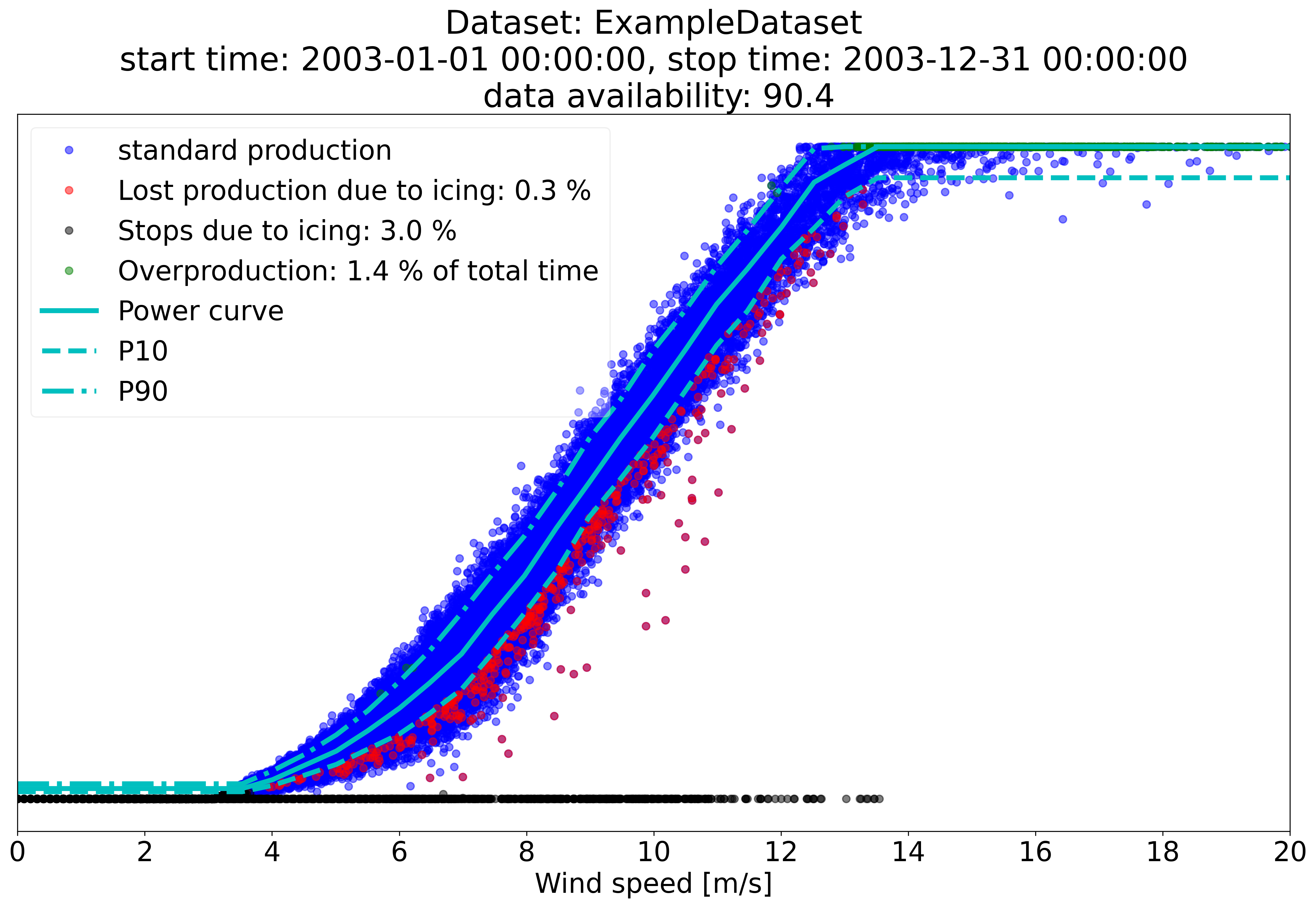
Figure 1:(ExampleDataset power curve scatter — blue: standard production, red: IEa losses (0.3%), black: IEb stops (3.0%), green: IEc overproduction (1.4% of total time))
8. Installation & Usage
8.1 Requirements
Python >= 3.6
numpy
scipy
matplotlib
sphinx   (optional, for documentation build)
The simplest way to set up the environment is with Anaconda, which bundles all required scientific Python libraries.
8.2 Installation
# Option 1: Clone the repository
git clone https://github.com/IEAWind-Task19/IceLossMethod.git
cd IceLossMethod

# Option 2: Install via pip
pip install t19_ice_loss
8.3 Configuration — The .ini File
All settings are defined in a plain-text .ini file. Each turbine has its own config file — this is a one-turbine-per-run tool. Below is the annotated configuration used for the ExampleDataset (2003), with every parameter explained:
[Source file]
id                  = ExampleDataset          # used to name all output files
filename            = ./fake_data2.csv
delimiter           = ,
quotechar           = NONE
datetime format     = %d.%m.%Y %H:%M         # matches "1.1.2003 0:00" format
datetime extra char = 0
fault columns       = 5,6,7,8                # cols with text values: Status, State, Ice detected, IPS
replace fault codes = True                   # must be True when status/state are text strings

[Output]
result directory    = ./results/example/
summary             = True    # overall statistics summary .txt
plot                = True    # power curve scatter plot saved as .png
alarm time series   = True    # per-timestamp icing alarm label (0/1/2/3) as .csv
filtered raw data   = True    # cleaned time series after air density correction
icing events        = True    # per-event start/stop/loss list as .csv
power curve         = True    # P10, P50, P90 reference table as .txt

[Data Structure]
timestamp index      = 0      # Timestamp
wind speed index     = 1      # Wind speed [m/s]
wind direction index = 2      # Wind direction [deg]
temperature index    = 3      # Ambient temperature [C]
power index          = 4      # output power [kW]
rated power          = 2000   # kW — this is a 2 MW turbine model
state index          = 5      # State column ("OK" = normal production)
normal state         = OK
site elevation       = 100    # metres above sea level — used for air density correction
status index         = 6      # Status column
status code stop value = STOP # value in Status column that means turbine is stopped

[Icing]
ice detection        = True   # an ice detector signal is present in the SCADA
icing alarm code     = WHAT   # value in the ice detector column that means ice detected
icing alarm index    = 7      # column 7: Ice detected
heating              = False  # no blade heating (IPS) at this site
ips status code      = ON
ips status index     = 8      # column 8: IPS (present in data but heating = False)
ips status type      = 1
ips power consumption index = -1   # no IPS power consumption signal in data

[Binning]
minimum wind speed      = 0
maximum wind speed      = 30   # m/s — extends to cut-out speed
wind speed bin size     = 0.5  # m/s — finer than the 1 m/s default
wind direction bin size = 360  # single global curve, no directional binning

[Filtering]
power drop limit        = 10   # P10 — lower threshold for IEa/IEb detection
overproduction limit    = 90   # P90 — upper threshold for IEc detection
icing time              = 3    # samples — event must persist ≥ 3 × 10 min = 30 min
stop limit multiplier   = 0.005 # 0.5% of rated power defines "turbine stopped"
stop time filter        = 6    # samples for IEb stop confirmation
statefilter type        = 1
stop filter type        = 1
power level filter      = 0.01 # removes obvious stoppages from the base dataset
reference temperature   = 3    # °C — only data above +3°C is used to build the reference curve
temperature filter      = 1    # °C — icing events are flagged when T < +1°C
min bin size            = 36   # minimum samples per bin = 36 × 10 min = 6 hours of data
distance filter         = True # additional smoothing pass on the power curve
start time              = NONE # no time restriction — use full dataset
stop time               = NONE
8.4 Running the Counter
python t19_counter.py ExampleDataset.ini
The script will execute Steps 1–3 in sequence and write all requested outputs to the results directory.
8.5 Processing Multiple Turbines
The code handles one turbine at a time. For a site with multiple turbines, create one .ini file per turbine and run the script separately for each:
python t19_counter.py turbine_WTG001.ini
python t19_counter.py turbine_WTG002.ini
python t19_counter.py turbine_WTG003.ini
Aggregating individual turbine results into farm-level statistics requires separate post-processing tools outside the scope of this package.
9. Example Results (ExampleDataset, 2003)
The ExampleDataset covers a full calendar year (2003) for a single wind turbine. Running the counter on this dataset produces the following output.
Key findings for the ExampleDataset (year 2003):
| Metric | Value |
|---|---|
| Data availability | 90.4% |
| Lost production due to icing (IEa) | 0.3% of reference |
| Stops due to icing (IEb) | 3.0% of reference |
| Overproduction hours (IEc) | 1.4% of total time |
The dataset illustrates the typical pattern seen at cold-climate sites: standstill losses (IEb) dominate over operational degradation losses (IEa). A turbine that has been forced to stop produces zero power for those hours, making IEb the larger component even when its event count is lower than IEa.
10. Further Development
This repository implements the IEA Task 19 ice loss method at the individual turbine level, strictly following the official Release 2.2 specification — intended as a clean, reproducible baseline.
The extensions below are developed as part of an my ongoing MSc thesis: “Icing Power Loss Forecasting for Wind Farms in Cold Climates Using Machine Learning” carried out at rebase.energy, Stockholm. They are not part of this repository and will be referenced here upon publication.
Extended Filtering Pipeline
An enhanced multi-layer filtering pipeline is built on top of the IEA baseline to improve reference curve purity across heterogeneous turbine models and multi-year SCADA archives. Details are confidential and will be disclosed upon thesis publication.
Wind Farm Aggregation
IEA Task 19 defines icing classes at the turbine level only, no farm-scale specification exists. The thesis addresses this directly, including signal aggregation logic and a majority-threshold label strategy to filter isolated single-turbine anomalies from genuine farm-wide icing events.
Machine Learning Integration
The IEA Task 19 output serves as ground truth for a downstream ML pipeline evaluating QRF, XGBoost, TCN, and the TIGER framework for day-ahead icing power loss forecasting.
Full results will be published upon thesis completion — June 2026.
11. References
- IEA Wind Task 19 (2019). Task 19 Ice Loss, Release 2.2. VTT Technical Research Centre of Finland. Author: Timo Karlsson — timo.karlsson@vtt.fi
- Repository: https://github.com/IEAWind-Task19/IceLossMethod
- License: BSD
IEA Wind. Cold Climate Wind Energy. https://iea-wind.org/task19/
- ISO 2533:1975. Standard Atmosphere. International Organization for Standardization. (Used for air density correction in the counter.)
Feedback and contributions are welcome. If you apply this method to your own site data, opening an issue with your findings helps improve the tool for the whole community.