K-Nearest Neighbours (KNN) Algorithm - Part 1

Source: step‑by‑step KNN guide by Utsav Desai on Medium.

1. Definition of KNN

K‑Nearest Neighbour (KNN) is a simple, non‑parametric machine learning algorithm that makes predictions based on the labels of the closest data points in the training set. It is supervised (it needs labeled examples) and can be used for both classification and regression tasks.

KNN assumes that points that are “close” in feature space tend to have similar labels or values. All training examples are stored; no explicit model is fitted in advance, which is why KNN is often called a lazy learner or instance‑based method.

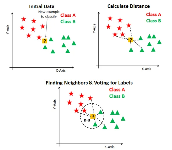
For a new input, the algorithm:

• Measures the distance between the new point and every point in the training data.
• Selects the $K$ closest points (the $K$ “nearest neighbours”).
• Classification: assigns the most common class among those neighbours.
• Regression: predicts the average (or weighted average) of their target values.

Because it makes very few assumptions about the data distribution, KNN is considered non‑parametric and can model complex decision boundaries if there is enough data and the features are well scaled.

2. What is “K” in K‑Nearest Neighbour?

The $K$ in K‑Nearest Neighbour is a hyperparameter that tells the algorithm how many neighbours to look at when making a prediction.

If $K = 1$, the algorithm uses only the single closest training point; the new point simply gets that neighbour’s label (for classification) or value (for regression).

For larger $K$ (3, 5, 10, …), the algorithm considers more neighbours, which smooths predictions.

• Very small $K$:
  • The decision boundary follows the training points very closely and can change a lot if one training sample changes.
  • This is low bias, high variance and usually risks overfitting, because the model chases noise in the training set.
• Larger $K$:
  • The prediction is an average over many neighbours.
  • The decision boundary becomes smoother and less sensitive to single noisy points.
  • This is higher bias, lower variance; the model may miss local structure and give overly “blurry” predictions.

When does KNN underfit?

Underfitting happens when $K$ is so large that KNN becomes too simple and cannot capture the true pattern in the data.

From the above explanation, choosing the value of $K$ should be done carefully.

There are some statistical methods for selecting $K$, including:

• Cross‑validation:
  Cross‑validation is a good way to find the best value of $K$. The dataset is split into $k$ folds. The model is trained on some folds and tested on the remaining ones, rotating which fold is used for testing. The $K$ that gives the highest average accuracy is usually chosen.

• Elbow method:
  In the Elbow Method a graph of error (or accuracy) versus different $K$ values is drawn. As $K$ increases, the error usually drops at first, then stops improving quickly. The “elbow” point where the curve bends is often a good choice.

• Odd values for $K$:
  For classification, using an odd number for $K$ helps avoid ties when deciding which class is most common among the neighbours.

Source: high‑level ideas adapted from a KNN article on GeeksforGeeks.

3. Distance metrics used in KNN

KNN needs a way to measure how similar or different two data points are, which is done with a distance metric in feature space. The choice of metric can significantly affect which points are considered neighbours and therefore the final predictions.

3.1 Euclidean distance

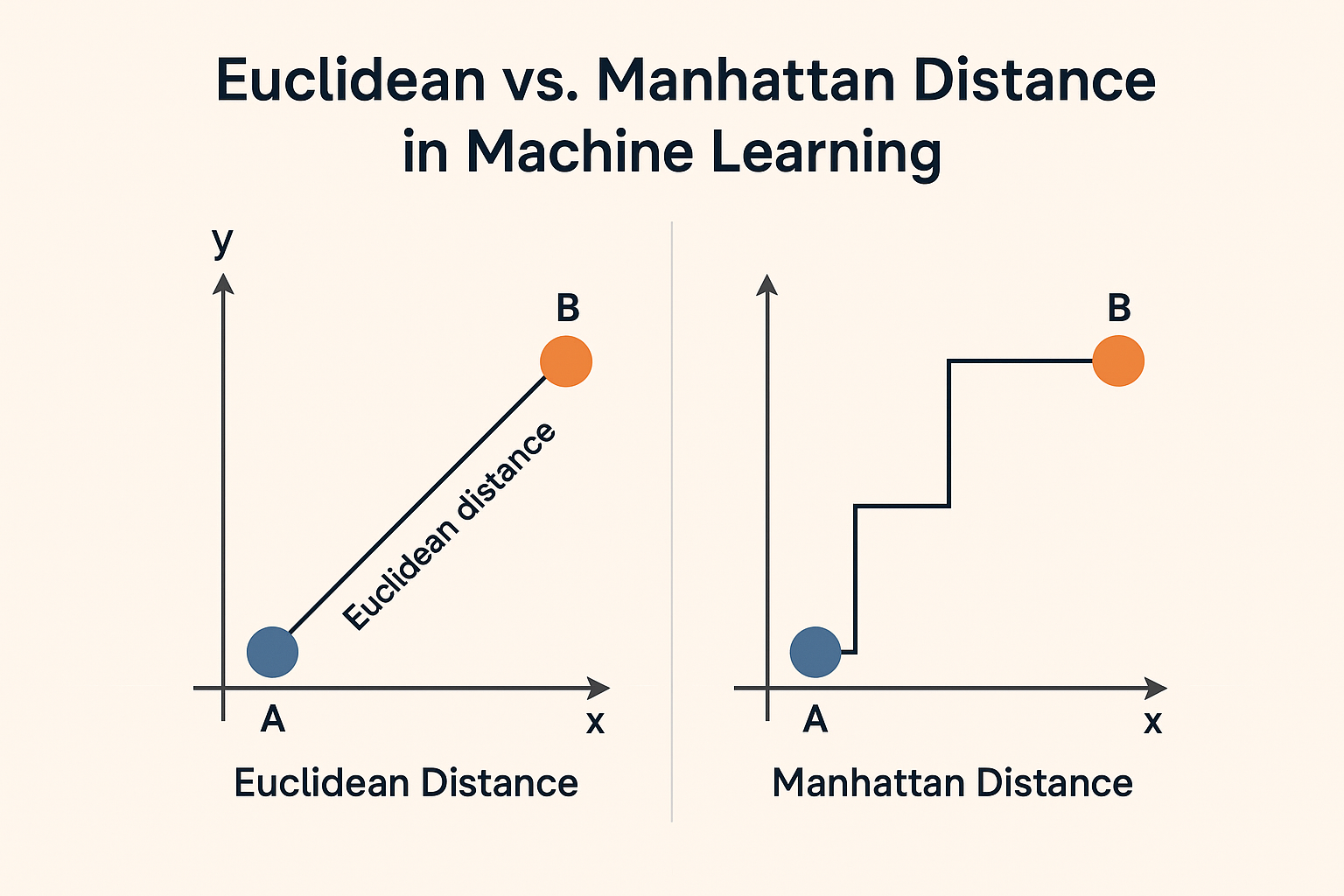
For two points \(x = (x_1, \dots, x_n), \quad y = (y_1, \dots, y_n),\)

the Euclidean distance is \(d_{\text{euclid}}(x, y) = \sqrt{\sum_{j=1}^{n}(x_j - y_j)^2}.\)

This is the usual straight‑line distance. It works well for continuous, scaled features.

3.2 Manhattan distance

Also called $L_1$ or city‑block distance: \(d_{\text{manhattan}}(x, y) = \sum_{j=1}^{n} \lvert x_j - y_j \rvert.\)

You can think of this as moving along a grid of streets instead of diagonally. It can be more robust to outliers than Euclidean distance.

3.3 Minkowski distance

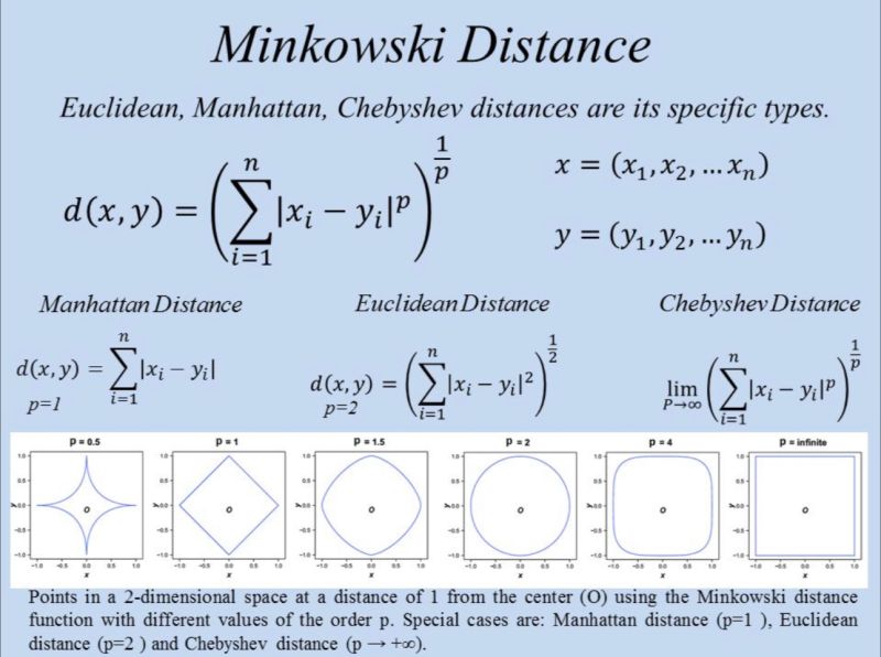
A general form that includes both Euclidean and Manhattan distances: \(d_{\text{minkowski}}(x, y) = \left(\sum_{j=1}^{n} \lvert x_j - y_j \rvert^p\right)^{1/p}.\)

• $p = 1$ → Manhattan distance
• $p = 2$ → Euclidean distance

By changing $p$, you control how strongly large differences are penalized.

3.4 Chebyshev distance

Chebyshev distance looks only at the largest coordinate difference: \(d_{\text{chebyshev}}(x, y) = \max_j \lvert x_j - y_j \rvert.\)

Two points are close only if all feature differences are small.

3.5 Cosine distance / similarity

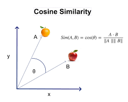
Cosine similarity says “how similar” two vectors are by comparing the angle between them.
A value close to 1 means the vectors point in almost the same direction (very similar),
0 means they are orthogonal (unrelated), and −1 means they point in opposite directions (very dissimilar).

The formula is

where:

• (x \cdot y) is the dot product (multiply each coordinate and sum).
• (\lVert x \rVert) and (\lVert y \rVert) are the lengths (norms) of the two vectors.

A common cosine “distance” turns similarity into a dissimilarity score:

Here, (\text{cosine_sim}(x, y)) is the similarity measure, and (d_{\text{cosine}}(x, y)) is 0 when vectors are identical in direction and grows as they become less aligned.

3.6 Distances for categorical data

For binary or categorical features, metrics like Hamming distance (fraction of positions that differ) or Jaccard distance (based on set overlap) are often better suited than Euclidean distance.

In practice, Euclidean distance is a good default for numeric, scaled features, but for text, binary attributes, or unusual feature structures, trying other metrics can improve KNN performance.