
Flappy bird Game Part 2 🐦 with Artificial Neural Network (ANN)
We often treat Machine Learning libraries like TensorFlow or PyTorch as “ Black bockes”. We feed data in, and magic come out. However, to have better understanding on deep learning, one must understand the mathematics happening under the hood.
For this project, I set out to buld an AI flappy bird based on Neuroevolution—the process of training Neural Networks using Genetic Algorithms (Darwinian Natural Selection).
There are three main steps in this projects:
- Step 1: Building a flappy bird game
- Step 2: Neural network
- Step 3: Natural selection algorithm
For the next coming parts, I will explain detailly every step.
Step 1: Creating a flappy bird game
Before an AI can learn, it needs a world to live in. In this step we build the “flappy bird” using the Pygame library. The main loop including:
- Input: Check for user/AI flap request.
- Physics: Update bird position ($\mathbf{v \leftarrow v + 0.7}$, $y \leftarrow y + v$).
- World Update: Move pipes, spawn new pipes, clean up old pipes.
- Scoring: Check the scoring condition (is the pipe past the bird?).
- Collisions: Check for death (Pipe or Floor).
- Drawing: Render the new scene.
1.1 The cordinate systems
The 1st thing to understad is the map. In mathclass, Y goes up. In computer graphics, Y goes down.
- (0,0): Top left corner of the screen.
- X increases: Moving right
- Y increases: Moving down (towards the floor).
- Y decreases: Moving up (toward the ceiling). In the code:
WINDOW_WIDTH = 900
WINDOW_HEIGHT = 600
FLOOR_Y = 512
We define the boundaries. The bird must stay between
Y=0(Ceiling) andY= 512(Floor).
1.2 Loading images
Next task is loading images for background, floor, bird animations frames and pipes. In terms of bird animation frames, we import three main animations to make bird moving his/her wings. For the drawing pipes, we import image for drawing bottom pipe and then flip it to draw top pipe.
# Background
background = pygame.image.load('assess/background-night.png').convert()
background = pygame.transform.scale(background, (WINDOW_WIDTH, WINDOW_HEIGHT))

# Floor
floor_img = pygame.image.load('assess/floor.png').convert()
floor_img = pygame.transform.scale(floor_img, (WINDOW_WIDTH, 100))

# Bird Animation Frames
bird_down = pygame.image.load('assess/yellowbird-downflap.png').convert_alpha()
bird_mid = pygame.image.load('assess/yellowbird-midflap.png').convert_alpha()
bird_up = pygame.image.load('assess/yellowbird-upflap.png').convert_alpha()
bird_list = [bird_down, bird_mid, bird_up]

# Pipes (Scaled and Flipped)
PIPE_IMG = pygame.image.load('assess/pipe-green.png').convert_alpha()
PIPE_IMG = pygame.transform.scale(PIPE_IMG, (70, 800)) # Scale tall to avoid stretching
PIPE_IMG_FLIPPED = pygame.transform.flip(PIPE_IMG, False, True) # Flip for top pipe
In here, to match the image pixel format with displya surface, and increase the render speed. We use convert() and .convert_alpha().
1.3 The pipe object (the obstacle)
The class Pipe defines the obstables that move across the screen.
a, Gap creation
When a new pipe is created, the vertial position of the gap is chosen randomly
safe_zone = 50
        min_gap_y = safe_zone
        max_gap_y = FLOOR_Y - safe_zone - self.opening
        self.gap_y = random.randint(min_gap_y, max_gap_y)
The gap must be within the safe zone, meaning it can not be too close the the floor FLOOR_Y = 512) or too close to the top edge. The zie of the gap itself (opening = 160) is fixed. The bottom pipe and top pipe are then created.
self.bottom_y = self.gap_y + self.opening
        self.top_height = self.gap_y
        self.bottom_height = FLOOR_Y - self.bottom_y
b, Pipe spawing logic
We can not draw a numerous of pipes that goes on forever. Computers will run out of memory. Instead, we use a “ Conveyor Belt” trick. The bird actually stays still horizontally (at x = 50). The world moves to the left.
The spawning logic
We keep a list of pipes pipes = [].
- Check distance: if the last pipe in the list far enough away?
if WINDOW_WIDTH - pipes[-1].x > PIPE_SPACING: - Spawn: if yes, create a new pipe at far right edge of the screen.
- Randomize: Pick a random height for the gap using
random.randint
The cleanup logic
If a pipe moves off the left side of the screen (x < -70), it is useless. We delete it from the list (pipe.pop(0)). This keep computer running fast because it never has to track more than 3 or 4 pipes at a time.
# Move pipes to the left
for pipe in pipes:
    pipe.update() # self.x -= GAME_SPEED

# Delete old pipes
if pipes[0].x < -pipes[0].width:
    pipes.pop(0)
1.4 The Physics of bird flying
We model the bird’s movement using simple opposing forces: constant gravity and an instant flap impulse.
Gravity
Gravity is implemented as a constant acceleration applied to the bird’s vertical speed (velocity, \(v\))
- Logic: In every single frame of the game, we increase the veritcal speed by a small, fixed amount (0.7). This makes the bird fall faster and faster.
- Mathematics & code: \(v_t+1 = v_t + 0.7 position Y_t+1 = Position Y_t + v_t+1\)
# In the Agent class, updated every frame:
self.vel += 0.7      # Gravity: Add to velocity every frame
self.y += self.vel   # Movement: Update position based on velocity
self.rect.y = int(self.y) # Update the hitbox
The flap (The counter-force)
When the AI decides to jump, we override gravity instantly.
- Logic: we don’t “add” upward force; we set the velocity to a negative number (-9). Since the Y-axis increases downward in Pygame, a negative velocity causes the bird to shoot upward.
- Mathematic & code: \(v_flap = 9\)
def flap(self):
  self.vel = -9  # Instant upward velocity
1.4 Scoring mechanism
In flappy bird, the score is not based on time, it is based on passing through pipes. The logic: passing a pope
- Fixed bird position: The bird’s horizontal position (
BIRD_X_POS = 50) is fixed. - Tracking: When a pipe is created, it has a boolean flag, passed = False.
- Score condition: The bird only scores when the pipe’s trailing edge has moved past the bird’s fixed X-position.
- One-time score: After the bird scores, the passed flag is immediately set to
True. This prevent the game from adding points continuously while the bird flies through the empty space between two pipes. The code for scoring is inplay_manuallyandrun_generationfor pipe in pipes: # ... (pipe movement and collision checks) # Scoring Check: if not pipe.passed and pipe.x + pipe.width < BIRD_X_POS: pipe.passed = True score += 1 # Crucial for Step 2/3 (AI Mode): # In run_generation, this line rewards ALL active agents: # agent.fitness += 101.5 Collision dection (the hitbox)
How do we know if the bird died? We use Rectangles (Rects). Every object in the game has an invisible box around it called a Hitbox. We ask the computer a simple geometry question: “Does Box A overlap with Box B?” In the Code: Pygame does the heavy math for us with colliderect: \(\text{Collision} \iff \text{Bird.Hitbox} \cap (\text{Pipe.TopHitbox} \lor \text{Pipe.BottomHitbox}) \ne \emptyset\)
# rect is the Bird's hitbox
# top_rect / bottom_rect are the Pipe's hitboxes
def collides(self, rect):
    # Check Top Pipe OR Bottom Pipe
    return rect.colliderect(top_rect) or rect.colliderect(bottom_rect)
Step 2: Artificial Neural Network
We don’t use “If/Else” statements to tell the bird how to play. We give it a brain and let it decide. We are not using a pre-built library like TensorFlow; we are building a raw mathematical model from scratch using Linear Algebra.
This is a Feed-Forward Neural Network. It takes information in, processes it through layers of math, and spits out a binary decision: Jump or Don’t Jump.
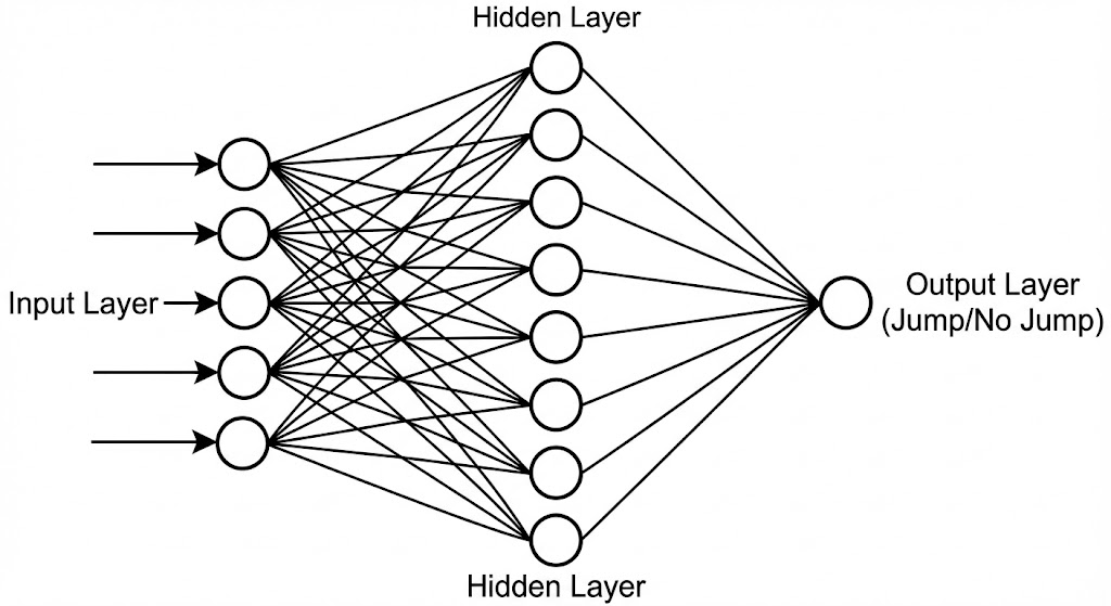
2.1 The architecture (topology)
The brain is structured in three layers. Data flows in one direction (Left to Right).
- Input layer (5 Neurons): The “Sensors”. These receive raw data from the game.
- Hidden layer (8 Neurons): The “Processors”. These neurons find patterns in the data (e.g., “The pipe is close AND I am too low”)
- Output layer (1 Neuron): The “Actuator”. It produces the final decision probability.
Code:
class NeuralNetwork:
    def __init__(self, layer_sizes=[5, 8, 1]):
        # ... initializes weights and biases based on layer_sizes
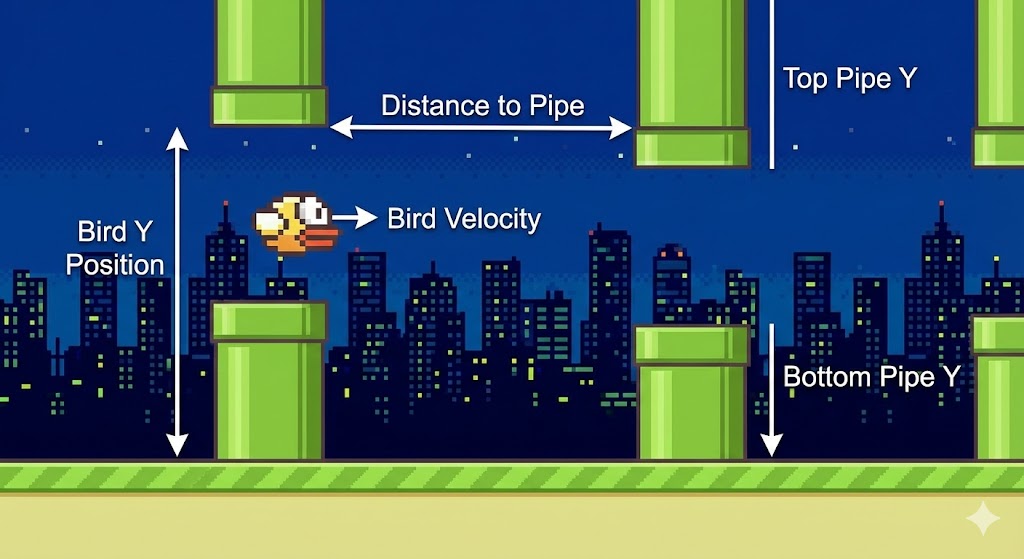
2.2 The input (The senses)
A neural network cannot understand “graphics.” It needs normalized numbers (usually between 0 and 1) to do math efficiently. This is essential because it prevents large numbers (like 500 for Y-position) from dominating the smaller numbers (like 0.7 for velocity) during the network’s calculations. In the Agent.think method, we feed it 5 specific numbers:
- Bird Y: $\frac{y}{height}$ (Where am I verticaly?)
- Bird Velocity: $\frac{vel}{20}$ (Am I falling fast?)
- Top Pipe Y: $\frac{top_y}{height}$ (Where is the ceiling danger?)
- Bottom Pipe Y: $\frac{bottom_y}{height}$ (Where is the floor danger?)
- Pipe Distance: $\frac{dist}{width}$ (How much time do I have?)
def think(self, bird_y, bird_vel, pipe_gap_top, pipe_gap_bottom, pipe_dist):
    inputs = np.array([[
        bird_y / WINDOW_HEIGHT,         # x1: Bird's Y-position (0 to 1)
        bird_vel / 20,                  # x2: Bird's Velocity/Direction
        pipe_gap_top / WINDOW_HEIGHT,   # x3: Top edge of the safe zone
        pipe_gap_bottom / WINDOW_HEIGHT,# x4: Bottom edge of the safe zone
        pipe_dist / WINDOW_WIDTH        # x5: Horizontal distance to pipe
    ]])
    return self.brain.forward(inputs)
2.3 The math: forward propagation
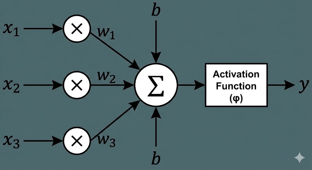
How does the brain turn those 5 numbers into a decision? It uses Matrix Multiplication.
Layer 1: Input $\rightarrow$ Hidden
First, the raw data travels from the sensors (Input Layer) to the processing unit (Hidden Layer).
a, The Weighted Sum (The Linear Step)
Every connection between an input and a neuron has a Weight ($W$). Think of weight as “importance”
- If a weight is high, the neuron pays close attention to that input.
- If a weight is zero, the neuron ignores it. The neuron multiplies every input by its weight, adds them all up, and adds a Bias ($B$). The bias is just a baseline offset—like a neuron’s “mood.” Some neurons might be naturally eager to jump (positive bias), while others are hesitant (negative bias). The Equation: \(Z_1 = (X \cdot W_1) + B_1\)
- $X$: The Input Vector ($1 \times 5$) containing our game data.
- $W_1$: The Weight Matrix ($5 \times 8$) linking inputs to hidden neurons.
- $B_1$: The Bias Vector ($1 \times 8$).
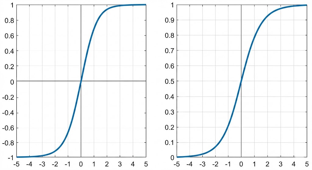
b. The Activation (Tanh)
The result of the math above ($Z_1$) can be any number—huge, tiny, or negative. To make sense of it, we need to “squash” it into a standardized range. For the hidden layer, we use the Hyperbolic Tangent (Tanh) function. \(H = \tanh(Z_1)\) Tanh is perfect here because it outputs numbers between -1 and 1.This allows the brain to understand negative relationships. For example, if the bird’s “Velocity” is a high positive number (falling fast), the brain can produce a strong negative signal (-1) that essentially says, “This is bad, we need to correct this.”
Layer 2: Hidden $\rightarrow$ Output
Now that the hidden neurons have processed the raw data into features (like “danger is close”), they pass that info to the final Output Neuron.
a. The Linear Step
We repeat the weighted sum process. The output neuron takes the results from the hidden layer ($H$), weighs them based on which hidden neurons are most trustworthy, and adds a final bias. \(Z_2 = (H \cdot W_2) + B_2\)2.
b. The Activation (Sigmoid)
For the final step, we don’t want a negative number. We are making a binary decision (Yes/No), so we want a probability between 0% and 100%. We use the Sigmoid function, which squashes any number into the range 0 to 1. \(\text{Output} = \frac{1}{1 + e^{-Z_2}}\) If the final number is > 0.5, the bird decides to flap. Otherwise, it keeps falling.
Code implementation:
def forward(self, x):
    # --- LAYER 1: Input to Hidden ---
    # 1. Matrix Multiply inputs by weights and add bias
    z1 = np.dot(x, self.weights[0]) + self.biases[0]

    # 2. Apply Tanh Activation
    # Squashes the result to [-1, 1]
    a1 = np.tanh(z1)

    # --- LAYER 2: Hidden to Output ---
    # 3. Matrix Multiply hidden results by weights and add bias
    z2 = np.dot(a1, self.weights[1]) + self.biases[1]

    # 4. Apply Sigmoid Activation
    # Squashes the result to [0, 1] for a probability
    output = 1 / (1 + np.exp(-z2))

    # --- DECISION ---
    # If the probability is > 50%, return True (JUMP)
    return output[0][0] > 0.5
2.4 Mutability and Copying
The final part of the NeuralNetwork class provides the tools necessary for the evolution process in Step 3. Code implementation:
def mutate(self, mutation_rate=0.1):
    # Randomly adds noise to weights and biases
    # ...
def copy(self):
    # Creates a perfect duplicate of the network
    # ...
Step 3: Genetic Algorithm (The evolution)
The Genetic Algorithm (GA) simulates the process of natural selection to optimize the weights and biases (the “genes”) of the Neural Networds. Instead of finding the perfect solution through complex math, the GA finds the best solution through trials, error, and survival of the fittest.
The learning framework can be shown:
| Generation | Action | Result |
| (G_n) | — | — |
| Play | 150 birds play the game. | We get 150 Fitness Scores. |
| Select | Sort by Fitness; save the top 10. | The best strategies survive. |
| Evolve | Clone the top performers; apply mutation. | New population (G_{n+1}) is created, slightly smarter than (G_n). |
| Repeat | Loop to the next generation. | Over many generations, the agents evolve a near-perfect strategy for playing Flappy Bird. |
3.1 Initializsation
The process begins in the evolve() function, which runs the simulation over many generations.
- Population Creation: We start with an initial group of agents. Each agent has a unique, randomly initialized brain. In this code, we create 150 unique birds, all with slightly different, random jumping habits.
population = [Agent() for _ in range(150)] - Simulation: The run_generation() function is the main game loop, where the entire population plays simultaneously.
- End Condition: A generation ends only when all 150 agents die (hitting a pipe, the floor, or the ceiling).
3.2 The fitness function (Evaluation)
Fitness is the quantitative measure of an agent’s success. It is the reward signal that tells the GA which agents are “good.”
Logic: How the Agent Earns Rewards An agent’s goal is to maximize its survival time and score.
| Reward Action | Fitness Increment | Code Reference |
|---|---|---|
| Survival | +0.1 per frame | agent.fitness += 0.1 (in run_generation loop) |
| Scoring | +10 per pipe passed | agent.fitness += 10 (when pipe.passed is set to True) |
The total fitness is calculated as: \(\text{Fitness} = (\text{Frames Survived} \times 0.1) + (\text{Pipes Passed} \times 10)\)
Goal: The heavy multiplier on the score (10) encourages the agents to pass pipes, while the time reward (0.1) encourages them to simply survive longer.
3.3 Selection (Survival of the Fittest)
After the generation ends, we identify the best-performing agents to be the parents of the next generation.
- Sorting: The entire population is sorted from best to worst based on their final fitness score.
population.sort(key=lambda x: x.fitness, reverse=True) - Elitism (Top Champions): The very best individuals are copied exactly into the new population. This ensures the best genetic material is never accidentally lost. The top 10 birds are granted eternal life (copied) into the next generation.
new_pop = []
for i in range(10): new_pop.append(population[i].copy())
3.4 Reproduction and Mutation
This is the creative phase where the new, potentially smarter generation is created by filling the remaining slots (140 agents).
The Code’s Role The remaining slots are filled by cloning and mutating brains from the top performers.
- Parent Selection: Agents are selected as parents from the top 30 performers (
population[:30]). Using a larger pool than just the top 10 introduces diversity.parent = random.choice(population[:30]) child = parent.copy() - Mutation: The copied brain (
child.brain) is slightly altered. This is the source of all improvement and diversity.child.brain.mutate(0.15) - Mutation Rate: The value 0.15 means there is a $15\%$ chance that any single weight or bias will be slightly altered.
- The Tweak: If a weight/bias is selected for mutation, a small amount of random Gaussian noise is added to it.
- \[\text{Weight}_{\text{new}} = \text{Weight}_{\text{old}} + (\text{RandomNoise} \times 0.5)\]
- This ensures that the brain doesn’t change drastically; it just jiggles a bit, leading to new behavioral strategies.
🌟 Wrapping up
And that’s the whole journey! We started with an empty screen and ended up with a bird that taught itself how to fly perfectly.
I hope you enjoy this code. Happy coding! 🎉
You can download the code through this link