Elastic Net Regression: Theory, Geometry, and Numerical Example

Elastic Net is a joint regularisation technique for linear regresson that combines the properties of both Lasso (L1) and Ridge (L2) penalties. By blending these two methods, it prevents overfitting, handles groups of correlated variables, and performs automated feature selection

The predicted value is:

Elastic Net Objective Function

The Elastic Net estimator solves:

Where:

• $y_i$: target value
• $\mathbf{x}_i$: feature vector
• $\boldsymbol{\beta}$: coefficient vector
• $n$: number of samples
• $\alpha$: regularization strength
• $\rho$: L1 ratio (mix between L1 and L2)
• $\lVert\boldsymbol{\beta}\rVert_1 = \sum_j \lvert\beta_j\rvert$: L1 norm
• $\lVert\boldsymbol{\beta}\rVert_2^2 = \sum_j \beta_j^2$: Squared L2 norm

Special Cases

• $\rho = 1$ → Lasso
• $\rho = 0$ → Ridge
• $0 < \rho < 1$ → Elastic Net blend

Alternative Form (sometimes used in papers)

Elastic Net can also be written as:

with:

Numerical Example

Let’s compute the Elastic Net loss for a simple regression problem.

1. Dataset & Parameters

• Number of samples ($n$): 3
• Features ($p$): 2
• Data Matrix ($X$): \(X = \begin{pmatrix} 1 & 2 \\ 2 & 1 \\ 1 & 1 \end{pmatrix}\)
• Target Vector ($y$): \(y = \begin{pmatrix} 3 \\ 3.5 \\ 2.5 \end{pmatrix}\)
• Hyperparameters: $\alpha = 0.1$, $\rho = 0.5$
  • $\lambda_1 = \alpha \rho = 0.05$
  • $\lambda_2 = \alpha (1 - \rho) = 0.05$

2. Candidate Coefficients

Assume a candidate coefficient vector: \(\boldsymbol{\beta} = \begin{pmatrix} 1.0 \\ 0.8 \end{pmatrix}\)

3. Step-by-Step Calculation

A. Predicted Values ($\hat{y} = X\boldsymbol{\beta}$)

• $\hat{y}_1 = 1(1.0) + 2(0.8) = 2.6$
• $\hat{y}_2 = 2(1.0) + 1(0.8) = 2.8$
• $\hat{y}_3 = 1(1.0) + 1(0.8) = 1.8$

B. Mean Squared Error (MSE) Term

\(\text{MSE Term} = \frac{1}{2n} \sum_{i=1}^{n} (y_i - \hat{y}_i)^2\)

• $y_1 - \hat{y}_1 = 3.0 - 2.6 = 0.4 \implies (0.4)^2 = 0.16$
• $y_2 - \hat{y}_2 = 3.5 - 2.8 = 0.7 \implies (0.7)^2 = 0.49$
• $y_3 - \hat{y}_3 = 2.5 - 1.8 = 0.7 \implies (0.7)^2 = 0.49$
• $\text{Sum of squared errors} = 0.16 + 0.49 + 0.49 = 1.14$
• $\text{MSE Term} = \frac{1}{2 \times 3} (1.14) = 0.19$

C. $L_1$ Regularization Term

\(\lambda_1 \|\boldsymbol{\beta}\|_1 = 0.05 \times (|1.0| + |0.8|) = 0.05 \times 1.8 = 0.09\)

D. $L_2$ Regularization Term

\(\frac{1}{2} \lambda_2 \|\boldsymbol{\beta}\|_2^2 = \frac{1}{2} \times 0.05 \times (1.0^2 + 0.8^2) = 0.025 \times 1.64 = 0.041\)

E. Total Elastic Net Loss

\(\text{Total Loss} = \text{MSE Term} + \lambda_1 \|\boldsymbol{\beta}\|_1 + \frac{1}{2} \lambda_2 \|\boldsymbol{\beta}\|_2^2\) \(\text{Total Loss} = 0.19 + 0.09 + 0.041 = 0.321\)

4. Minimizing the Loss (How to reduce it)

To minimize the total loss, we optimization-solve for the best coefficient vector $\boldsymbol{\beta}^*$ (typically via Coordinate Descent or gradient-based algorithms).

For this specific configuration, the optimal coefficients are: \(\boldsymbol{\beta}^* \approx \begin{pmatrix} 1.303 \\ 0.868 \end{pmatrix}\)

Recalculating the loss components with $\boldsymbol{\beta}^*$:

• Predictions: $\hat{y}_1 \approx 3.039$, $\hat{y}_2 \approx 3.474$, $\hat{y}_3 \approx 2.171$
• MSE Term: $\frac{1}{6} \left( (3 - 3.039)^2 + (3.5 - 3.474)^2 + (2.5 - 2.171)^2 \right) \approx 0.018$
• $L_1$ Penalty: $0.05 \times (1.303 + 0.868) \approx 0.109$
• $L_2$ Penalty: $0.025 \times (1.303^2 + 0.868^2) \approx 0.061$

\(\text{Minimum Loss} \approx 0.018 + 0.109 + 0.061 = 0.188\) Finding the optimal $\boldsymbol{\beta}^*$ successfully reduces the loss from 0.321 to 0.188.

The Grouping Effect (Grouped Selection)

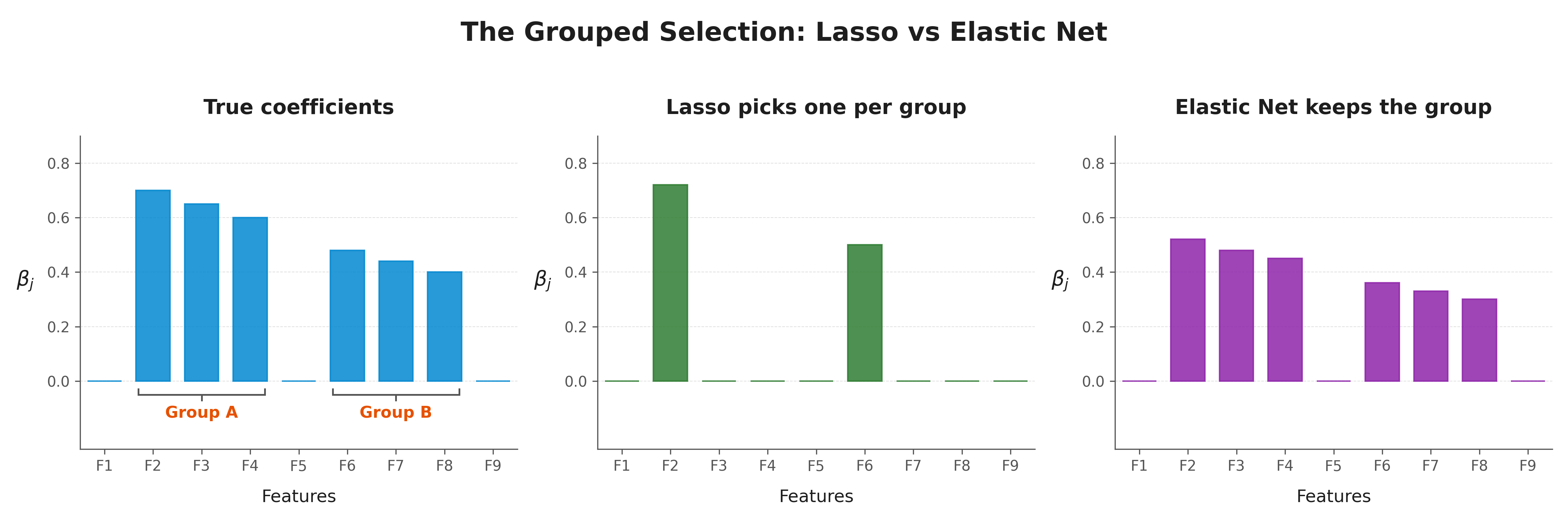
A major weakness of Lasso regularization is how it handles strongly correlated features (features that form a group of related variables). When presented with a group of highly correlated variables, Lasso tends to arbitrarily select only one variable from the group and drop (zero out) all the others. This can lead to model instability and loss of relevant context.

Elastic Net overcomes this limitation. By blending the $L_1$ and $L_2$ penalties, the $L_2$ component forces the coefficients of correlated features to shrink together, allowing Elastic Net to perform grouped selection (either keeping or dropping the whole group together).

Below is the visualization of this grouping behavior across 3 panels:

Geometric Representation

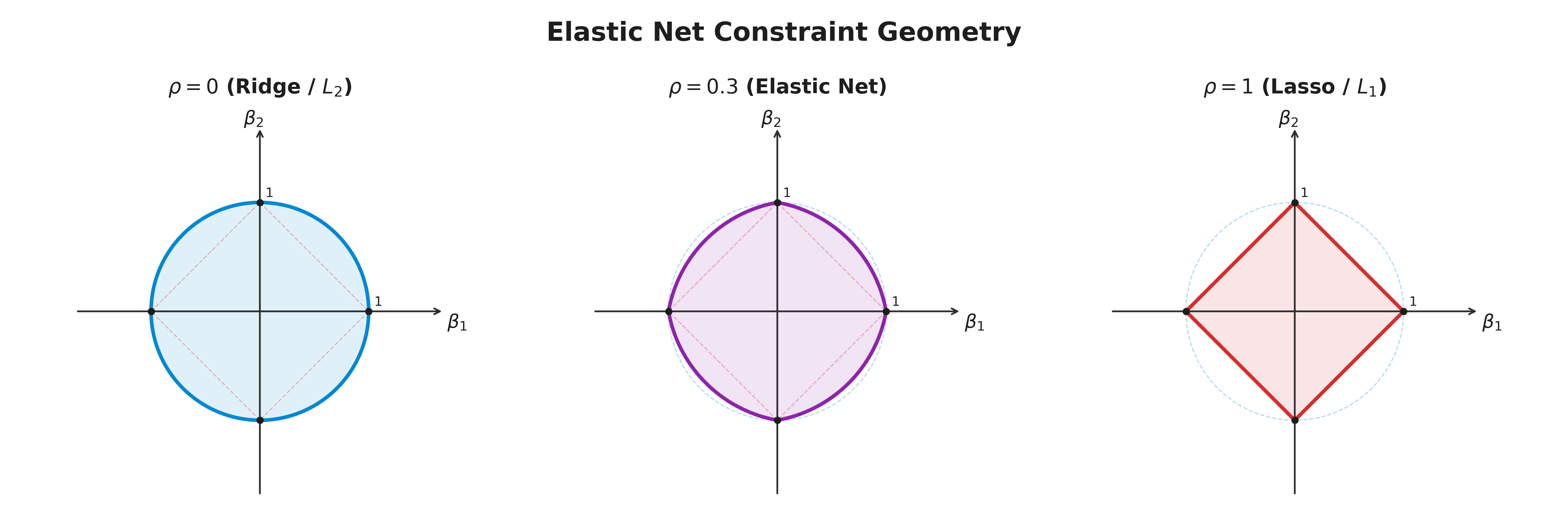
When plotted on a Cartesian Plane the elastic net falls in between the ridge and lasso regression plots since it is the combination of those two regression methods. The plot for the elastic net also exhibits singularity at the vertices, which are important for sparsity. It also exhibits strict convex edges where the convexity depends on the value of $\rho$.