
Support Vector Machine - Methodology 🧭
Series: Machine Learning Algorithms Part: 1 of 2 (Theory)
1. What is a Support Vector Machine?
Support Vector Machines (SVMs) are a supervised learning algorithm introduced by Vapnik (1992) for both classification and regression tasks. SVMs work by finding the optimal hyperplane that separates data points into different classes. Their power comes from constructing a boundary that maximises the margin between classes. A larger margin generally leads to better generalisation performance.
Beyond the mathematics, SVMs can be understood intuitively: imagine two cities on a map and you must build the widest possible highway between them without touching any buildings. The buildings closest to the highway determine its position. These buildings are the support vectors.
2. Key Terms
Hyperplane: A decision boundary that separates data points into different classes in a high-dimensional space. In 2D it is a line; in 3D it is a plane. In $N$-dimensional space, a hyperplane has $N-1$ dimensions.
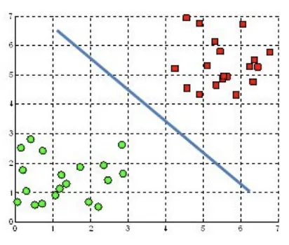 Figure: Illustration of the SVM hyperplane in 2D (Source: Kristori, 2023)
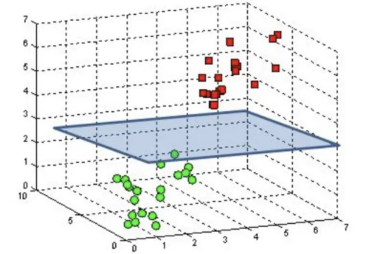 Figure: Illustration of the SVM hyperplane in 3D (Source: Kristori, 2023)
Margin: The distance between the hyperplane and the closest data points from each class. SVM aims to maximise this margin for a more robust classifier.
Support vectors: The data points lying closest to the decision boundary. They determine the position and orientation of the hyperplane and have a significant impact on classification accuracy. SVMs are named after these points because they “support” or define the decision boundary.
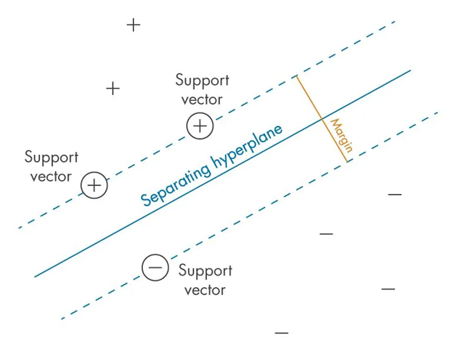 Figure: Illustration of the SVM margin and support vectors in 2D (Source: Singh, 2023)
Weight vector: The vector $\mathbf{w}$ is perpendicular to the hyperplane and determines its orientation. Its direction indicates how the hyperplane is oriented and its magnitude determines how steep the separation boundary is.
3. Linear vs Non-Linear SVM
Linear SVM
Where data is linearly separable, a linear SVM finds a straight line or hyperplane that best separates the classes. In wind power, a linear rule might be: “If the temperature is below 0°C, the turbine is iced.” However, icing is more complex than that since it depends on the combination of temperature, specific humidity, and wind speed.
Non-Linear SVM
Real-world data is often not linearly separable. When no straight line can separate classes, the data must be transformed into a higher-dimensional space where separation becomes possible. The classes are said to be linearly inseparable in the original feature space.
 Figure: Examples of linearly inseparable data that require transformation into a higher-dimensional space (Source: Singh, 2023)
4. Why Explicit Transformation Fails: Four Problems
To understand why the kernel trick is needed, it helps to work through four problems that make explicit high-dimensional transformation infeasible.
Problem 1: Concentric vs Non-Concentric Clusters
The difficulty of separation depends entirely on the shape of the clusters.
For a concentric case (such as a bullseye pattern), separation requires only one reference point. Each point’s distance from the centre determines its class: $Z = \sqrt{X^2 + Y^2}$. In 3D with this new feature, the classes separate perfectly with a flat plane.
For a non-concentric case (such as icing events scattered across three separate clusters in feature space), measuring from a single origin is no longer enough. The algorithm must evaluate for every data point its distance to every other point. In SCADA data, icing events form exactly this non-concentric structure, clustering at specific combinations of AmbientTemperature, RelativeHumidity, and ws_corrected.
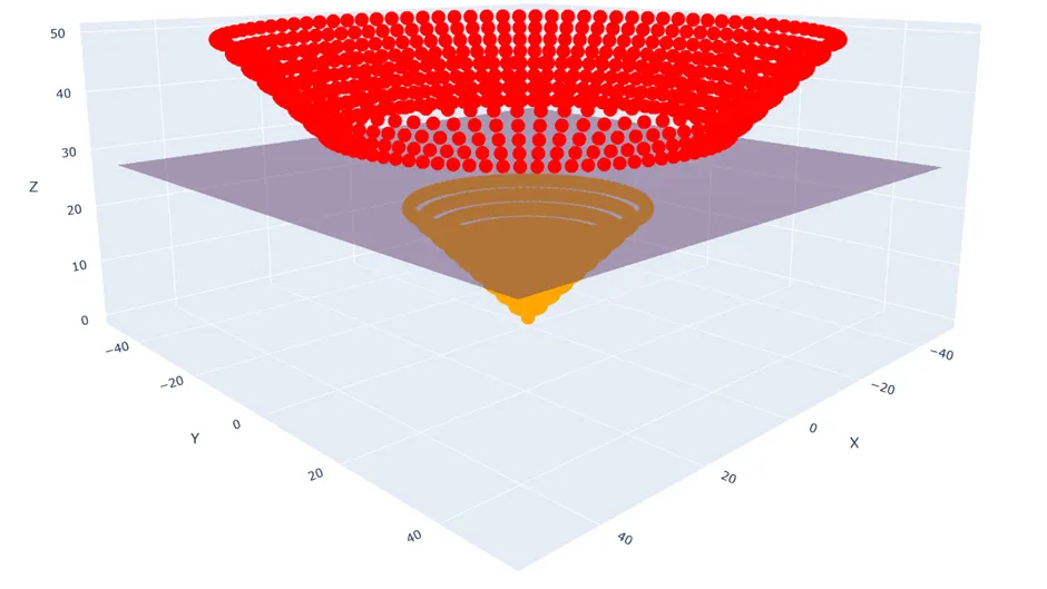 Figure: Concentric classes (left) separable by distance from origin. The same points lifted into 3D with $Z = \sqrt{X^2 + Y^2}$ become linearly separable by a flat plane (Source: Singh, 2023)
Problem 2: The Pairwise Distance Problem
The pairwise comparison requirement is known as the pairwise distance problem. Given $n$ items, the number of unique pairs is:
\[\frac{n(n-1)}{2} \approx \frac{n^2}{2}\]With only 10,000 rows of SCADA data (a tiny dataset by this study’s standards), the number of pairwise comparisons is already approximately 50 million distance calculations for a single feature. With 50 features, the total reaches billions of operations, making explicit transformation computationally infeasible.
Problem 3: Time Complexity
$O(n^2)$ time complexity describes how computation time grows as data grows:
| Complexity | What It Means | Real Example |
|---|---|---|
| $O(n)$, Linear | 2x more data: 2x slower | Scanning a list |
| $O(n \log n)$ | 2x more data: just over 2x slower | Sorting a list |
| $O(n^2)$, Quadratic | 2x more data: 4x slower; 10x: 100x slower | Pairwise distances |
As the SCADA dataset grows from one month (~10K rows) to three years (~3.47M rows), computation time scales by a factor of roughly 120,000.
Problem 4: Choosing the Right Transformation
Even if the computational cost were acceptable, a second problem remains: which transformation is correct? For just two features $X$ and $Y$ with degree-2 polynomials, the candidates are $X$, $Y$, $XY$, $X^2$, $Y^2$, giving 10 possible 3D feature combinations. Not all combinations produce a separable space. With 50 SCADA features and degree-3 terms included, the number of possible polynomial combinations is astronomically large.
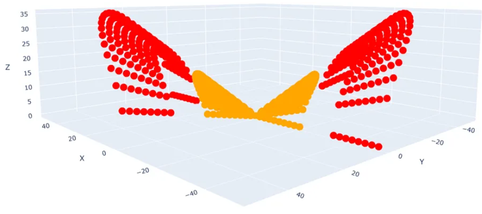 Figure: $X$ vs $Y$ vs $XY$ plot of the same data. This feature combination is not linearly classifiable (Source: Singh, 2023)
5. The Kernel Trick: Solution to All Four Problems
Instead of explicitly finding a transformation function $\phi(\mathbf{x})$ to project data into a higher-dimensional space, the algorithm uses the Kernel Trick. This method computes the similarity between the images of the data points directly. Rather than calculating $\phi(\mathbf{x}{i})$ and $\phi(\mathbf{x}{j})$ individually, a kernel function $K$ computes their dot product in the new feature space:
\[K(\mathbf{x}_{i}, \mathbf{x}_{j}) = \langle \phi(\mathbf{x}_{i}), \phi(\mathbf{x}_{j}) \rangle\]This approach allows the model to learn complex non-linear decision boundaries while avoiding the computational “curse of dimensionality.”
The three standard kernel functions are:
Linear Kernel:
\[K(\mathbf{x}_{i}, \mathbf{x}_{j}) = \mathbf{x}_{i}^{T} \mathbf{x}_{j}\]Polynomial Kernel:
\[K(\mathbf{x}_{i}, \mathbf{x}_{j}) = (\gamma \mathbf{x}_{i}^{T} \mathbf{x}_{j} + r)^{d}\]RBF Kernel (Gaussian):
\[K(\mathbf{x}_{i}, \mathbf{x}_{j}) = \exp(-\gamma \| \mathbf{x}_{i} - \mathbf{x}_{j} \|^{2})\]In these equations:
- Hyperparameter $\gamma$ (Gamma): Determines the “reach” or influence of a single data point. A high $\gamma$ makes the model focus only on nearby points, creating complex boundaries (prone to overfitting). A low $\gamma$ produces smoother, more generalised boundaries.
- Parameter $r$ (Coefficient): Controls the influence of higher-degree versus lower-degree polynomials within the polynomial kernel.
- Parameter $d$ (Degree): The power to which the polynomial is raised, defining the complexity of the feature space.
The RBF kernel computes a similarity score that decays exponentially based on squared Euclidean distance: two points that are close together receive a score near 1, while points far apart receive a score approaching 0. Crucially, the RBF kernel implicitly maps data into an infinite-dimensional feature space, enabling arbitrarily smooth and complex boundaries without specifying an exact polynomial combination.
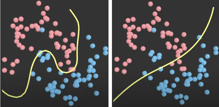 Figure: Effect of $\gamma$ on the RBF kernel decision boundary. Left ($\gamma = 1$): tightly curved, matches data locally. Right ($\gamma = 0.01$): smooth and near-linear (Source: Singh, 2023)
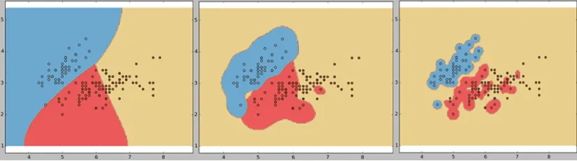 Figure: Three models with different $\gamma$ values. Left ($\gamma = 0.1$): well fitted. Middle ($\gamma = 10$): overfitted. Right ($\gamma = 100$): extremely overfitted (Source: Singh, 2023)
Key Insight: The RBF kernel is selected for icing studies because icing events form localised, non-concentric clusters in the
AmbientTemperaturexRelativeHumidityxws_correctedfeature space. Linear and polynomial kernels impose structural assumptions that a physically threshold-driven, multi-condition phenomenon like icing does not satisfy.
6. Soft Margin: Handling Noise and Overlap
Hard Margin (Ideal World)
If data were perfectly separable with no noise, the hard margin SVM would demand zero violations: every training point must sit on the correct side of the margin boundary. Two problems arise immediately. First, a single misplaced point (such as a faulty anemometer reading that looks like icing) would either prevent the SVM from finding a solution or force a narrow, distorted margin. Second, when classes genuinely overlap (as icing and non-icing conditions do near 0°C), no hard margin exists at all.
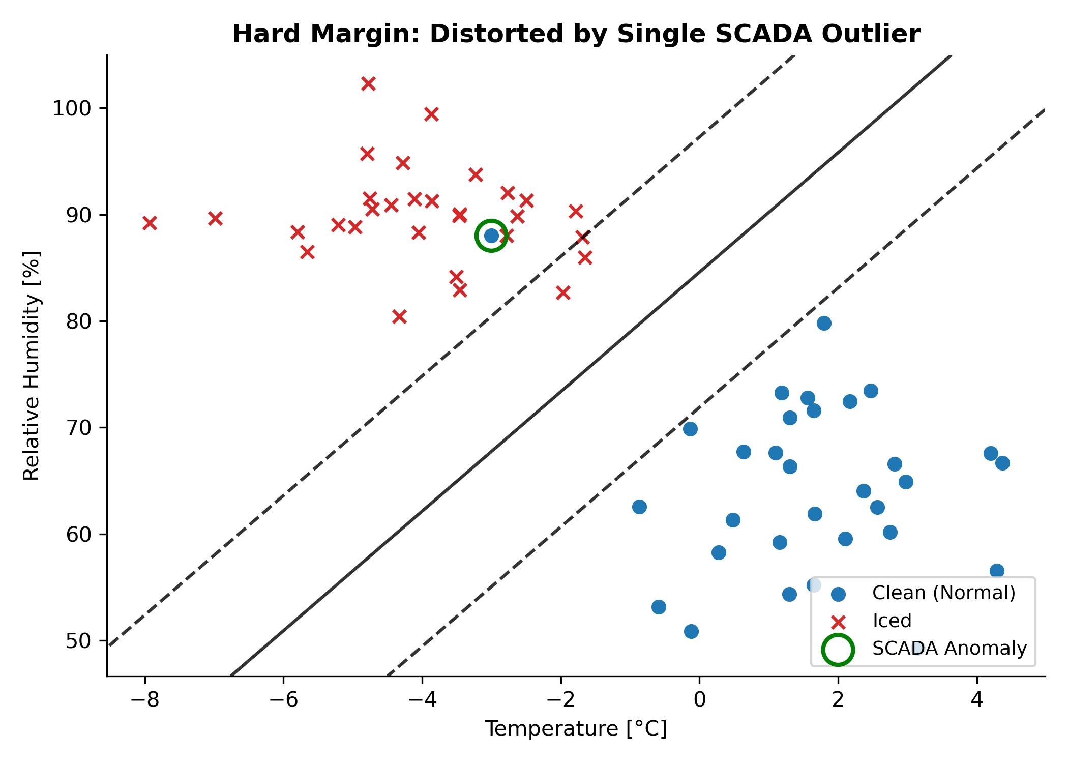 Figure: A single outlier introduced into the left class completely distorts the hard-margin decision boundary, misclassifying non-outlier data.
Soft Margin (Real World)
The soft margin SVM introduces slack variables $\xi_{i} \geq 0$ for each training point. A slack variable measures how far a point is on the wrong side of its class margin boundary. The trade-off is controlled by the regularisation parameter $C$:
\[\min_{\mathbf{w}, \beta_{0}, \boldsymbol{\xi}} \quad \frac{1}{2} \|\mathbf{w}\|^{2} + C \sum_{i=1}^{n} \xi_{i} \tag{3.16}\]Rather than forcing a narrow road because one building blocks the path, the soft margin allows a small number of misclassifications so that a wider, more robust boundary can be constructed.
| $C$ Value | Behaviour | Risk |
|---|---|---|
| Very high (e.g., 1000) | Almost hard margin, penalises every violation severely | Overfits; boundary hugs training data too closely |
| High (e.g., 100) | Narrow margin, few misclassifications | May overfit to noise |
| Moderate (e.g., 1 to 10) | Balanced margin width vs misclassifications | Generally best generalisation |
| Low (e.g., 0.1) | Wide margin, many misclassifications tolerated | May underfit |
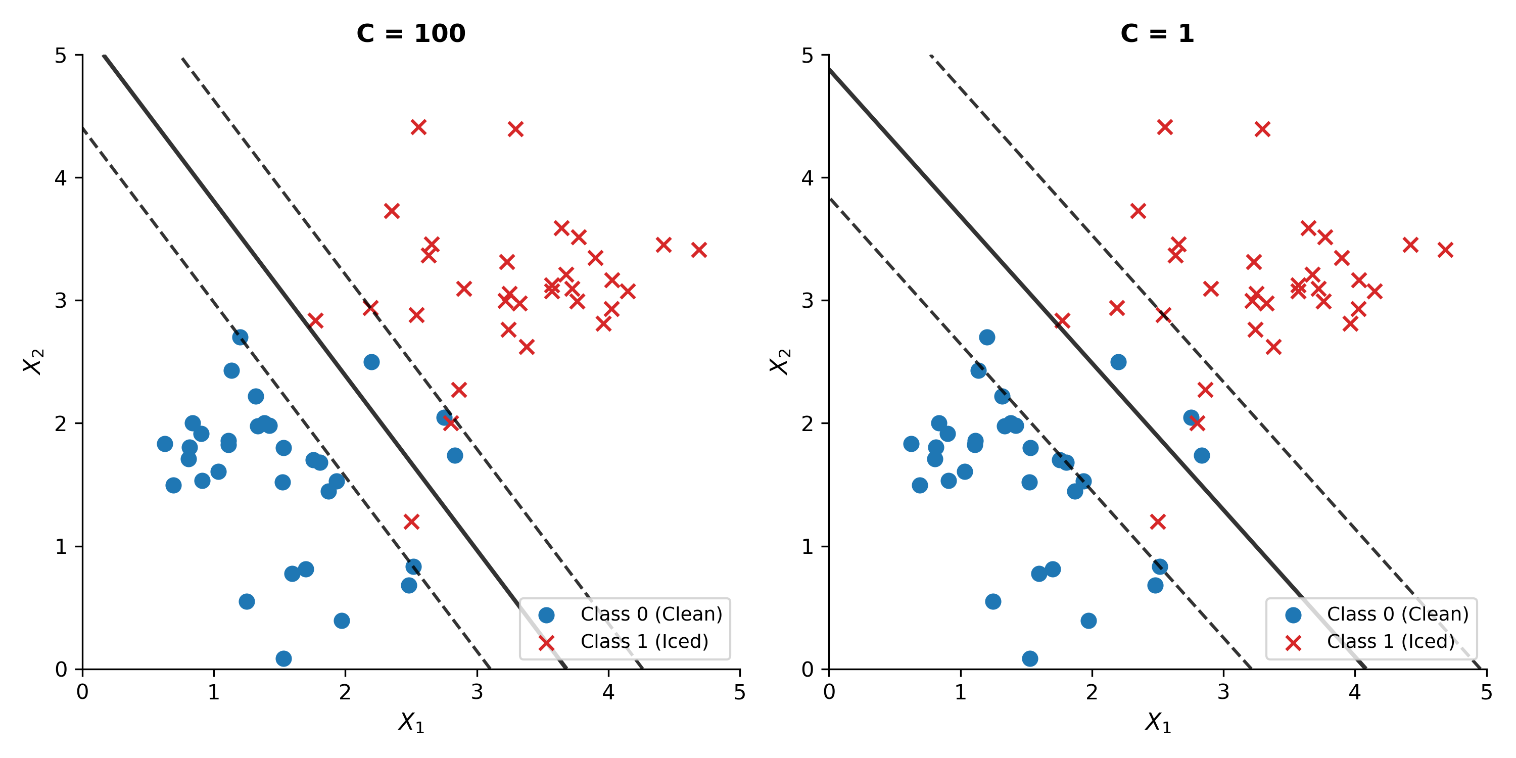 Figure: Same dataset with $C = 100$ (left, narrow margin) vs $C = 1$ (right, wider margin with better generalisation).
Key Insight: $C$ controls the bias-variance trade-off. High $C$ gives low bias and high variance. Low $C$ gives high bias and low variance. A moderate $C$ is appropriate for SCADA data because it tolerates transient anomalies (a single timestep where an anemometer stalls) without sacrificing overall icing detection.
7. From Classification to Regression: The SVR Tube
Where SVM for classification finds the widest street separating two classes, Support Vector Regression (SVR) inverts this idea. Instead of a highway between two classes, SVR fits a tube around the data. The goal is to include as many points as possible inside the tube while keeping it as narrow as possible.
Step 1: Define the $\varepsilon$-Insensitive Tube
SVR defines a tube of half-width $\varepsilon$ around the regression surface. Any data point falling inside the tube incurs zero penalty. Only points outside the tube generate an error and influence the model.
In wind power forecasting, $\varepsilon$ represents the threshold of acceptable prediction error. Minor fluctuations in loss_kw due to turbulence or measurement noise fall inside the tube and are ignored. Severe icing-induced losses that exceed $\varepsilon$ become the support vectors that drive the model’s fitting effort.
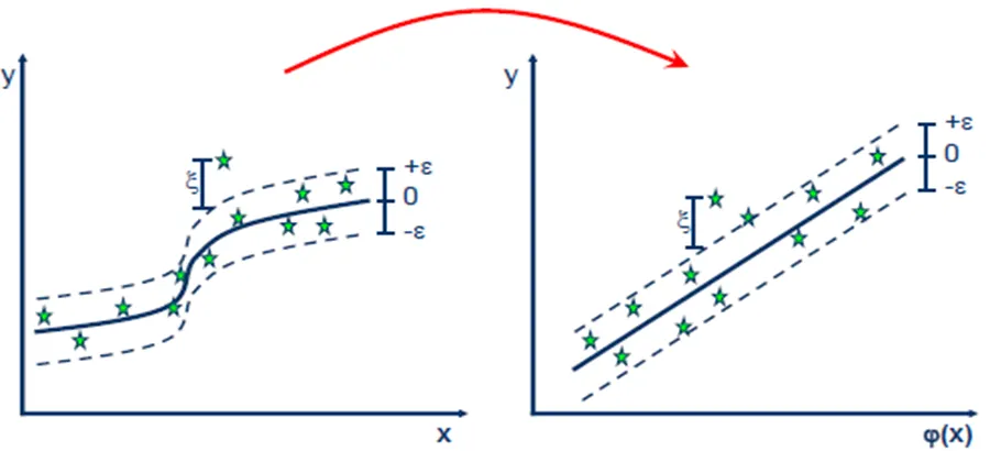 Figure: SVR regression surface surrounded by the $\varepsilon$-insensitive tube. Points inside have zero loss; points outside become support vectors (Source: Singh, 2023)
Step 2: Soft Margin Tolerance
Just as SVM uses slack variables for classification, SVR uses two slack variable sets: $\xi_{i} \geq 0$ for points above the tube and $\xi_{i}^{*} \geq 0$ for points below. The SVR optimisation problem is:
\[\min_{\mathbf{w}, \beta_{0}, \boldsymbol{\xi}, \boldsymbol{\xi}^{*}} \quad \frac{1}{2} \|\mathbf{w}\|^{2} + C \sum_{i=1}^{n} (\xi_{i} + \xi_{i}^{*}) \tag{3.17}\]subject to:
- $y_{i} - (\mathbf{w}^{T} \mathbf{x}{i} + \beta{0}) \leq \varepsilon + \xi_{i}$
- $(\mathbf{w}^{T} \mathbf{x}{i} + \beta{0}) - y_{i} \leq \varepsilon + \xi_{i}^{*}$
- $\xi_{i}, \xi_{i}^{*} \geq 0$
Step 3: Apply the Kernel Trick
For non-linear icing relationships, the kernel trick is applied identically as for classification. The SVR prediction function becomes:
\[f(\mathbf{x}) = \beta_{0} + \sum_{i=1}^{n} (\alpha_{i} - \alpha_{i}^{*}) \, K(\mathbf{x}, \mathbf{x}_{i}) \tag{3.18}\]where $\alpha_{i}$ and $\alpha_{i}^{}$ are Lagrangian multipliers for each training point’s deviation above and below the tube. Points inside the tube have $\alpha_{i} = \alpha_{i}^{} = 0$ and contribute nothing to the prediction. The constraints are:
\[\sum_{i=1}^{n} (\alpha_{i} - \alpha_{i}^{*}) = 0, \quad 0 \leq \alpha_{i} \leq C, \quad 0 \leq \alpha_{i}^{*} \leq C \tag{3.19}\]Step 4: Final Prediction
Prediction for a new data point $\mathbf{x}^{*}$ uses only the support vectors:
\[\hat{y} = \beta_{0} + \sum_{i \in \text{SV}} (\alpha_{i} - \alpha_{i}^{*}) \, K(\mathbf{x}^{*}, \mathbf{x}_{i}) \tag{3.20}\]The sum runs only over the support vectors. All other training points have zero contribution. This sparsity is a fundamental advantage: after training, adding new data points that fall inside the tube does not change the model at all.
Key Insight: During non-icing periods
loss_kw$\approx 0$. These timesteps fall inside the $\varepsilon$-tube and generate zero penalty. During icing eventsloss_kwis large; these points fall outside the tube and become the support vectors driving the model. SVR naturally concentrates its fitting effort on the operationally critical high-loss timesteps.
8. Computational Constraint
SVR’s kernel matrix $K(\mathbf{x}{i}, \mathbf{x}{j})$ must be evaluated for all $n(n-1)/2$ pairs of training points, giving training complexity of $O(n^{2})$ to $O(n^{3})$. As the SCADA dataset grows from one month (~10K rows) to three years (~3.47M rows), computation time scales by a factor of roughly 120,000. SVR is therefore applied only at farm scale and on a stratified 10% turbine subsample that preserves the icing/non-icing ratio.
| Dataset | Size | SVR Feasibility |
|---|---|---|
| Farm scale (Track 2) | ~106,500 rows | Feasible, applied directly |
| Turbine scale (Track 1) | ~3.47M rows | Infeasible, quadratic complexity |
| Turbine scale, 10% subsample | ~347,000 rows | Feasible with stratified sampling |
9. SVR vs Tree-Based Methods
| Property | Random Forest | XGBoost | SVR |
|---|---|---|---|
| Learning approach | Parallel ensemble trees | Sequential ensemble trees | Single optimal surface |
| Non-linearity | Axis-aligned splits | Axis-aligned splits | Kernel trick: smooth mapping |
| Decision boundary | Blocky, step-shaped | Blocky, step-shaped | Smooth, curved |
| Training complexity | $O(n \log n)$ per tree | $O(n \log n)$ per tree | $O(n^{2})$ to $O(n^{3})$ |
| Feature scaling | Not required | Not required | Mandatory |
| Missing values | Requires imputation | Native handling | Requires imputation |
| Feature importance | Gini + SHAP | Gain + SHAP | None built-in |
| Regularisation | Implicit (averaging) | Explicit L1/L2 | $C$ + $\varepsilon$ tube |
| Solution type | Average of many trees | Sum of residual corrections | Sparse support vectors |
| Overfitting control | Variance reduction | Regularised boosting | Maximum margin + $C$ |
SVR’s smooth curved boundaries via the RBF kernel may better capture the continuous physical transition of ice formation (the gradual aerodynamic degradation as ice accretes on blades) compared to the blocky, axis-aligned splits of RF and XGBoost. However, this potential advantage must be weighed against the computational constraint that limits SVR to a 10% subsample at turbine scale.
10. Advantages and Limitations
Advantages
- Smooth non-linear boundaries. The RBF kernel produces smooth curved boundaries that match the continuous physics of ice accretion, not abrupt axis-aligned jumps.
- Robust to outliers. The soft margin tolerates individual noisy SCADA readings without distorting the global boundary.
- Sparse solution. Only support vectors define the model. Adding new non-support points after training changes nothing, making inference memory-efficient.
- Globally optimal. SVR solves a convex quadratic programme. The solution cannot get stuck in local minima, unlike gradient descent methods.
- Well-defined regularisation. $C$ and $\varepsilon$ have clear geometric interpretations that connect directly to physical concepts.
- Handles class imbalance naturally. SVR focuses on the hardest points (the support vectors at the icing boundary), where operational decisions matter most.
Limitations
- Quadratic complexity. $O(n^{2})$ to $O(n^{3})$ training makes SVR infeasible at full turbine scale without subsampling.
- Mandatory feature scaling. Forgetting standardisation renders the RBF distance metric meaningless. RF and XGBoost require no scaling.
- No native missing value handling. SCADA gaps must be imputed before training, an extra preprocessing step that XGBoost handles natively.
- No built-in feature importance. SHAP Kernel Explainer works but is far slower than Tree SHAP used for RF and XGBoost.
- Sensitive to hyperparameters. The $C$, $\varepsilon$, $\gamma$ interaction is non-trivial. A poorly tuned SVR can underperform a default RF.
- Black-box. The model is defined by kernel evaluations over support vectors with no human-readable decision rules.
11. Conclusion
Support Vector Machines offer a geometrically principled approach to both classification and regression. The kernel trick elegantly solves the problem of non-linear separation without the computational cost of explicit high-dimensional transformation. The soft margin and slack variables make the algorithm robust to real-world noise and class overlap. For regression tasks like icing power loss forecasting, SVR’s $\varepsilon$-insensitive tube naturally focuses the model’s attention on operationally critical high-loss events while ignoring small measurement fluctuations.
The main trade-off is computational: quadratic training complexity limits SVR to subsampled or farm-scale datasets, while tree-based methods scale more easily to millions of rows.
In the next post, we will present the practical application of SVR using Python, including kernel selection, hyperparameter tuning, and feature scaling.
References
- Vapnik, V. (1995). The Nature of Statistical Learning Theory. Springer. https://doi.org/10.1007/978-1-4757-3264-1
- Singh, S. (2023). Support Vector Machine: A Practical Guide. Medium article
- Kristori (2023). SVM Hyperplane Illustrations. Referenced from course materials.
- Tibrewal, K. (2023). Introduction to SVR. Medium article