
Random Forest - Methodology 🌲
Series: Machine Learning Algorithms Part: 1 of 2 (Theory)
1. What is Random Forest?
Random Forest (RF) is a powerful ensemble learning method used for both classification and regression. It was first introduced by Breiman (2001). By combining many decision trees, it improves accuracy and reduces the risk of overfitting.
The key idea is that a group of weak learners (individual trees) can together form a strong learner (the forest). Each tree is built on a different random sample of the data, so the trees make different errors. When their outputs are combined, the errors cancel out and the overall prediction becomes more stable and accurate.
- For classification, the final prediction is the majority vote.
- For regression, the final prediction is the average of all tree outputs.
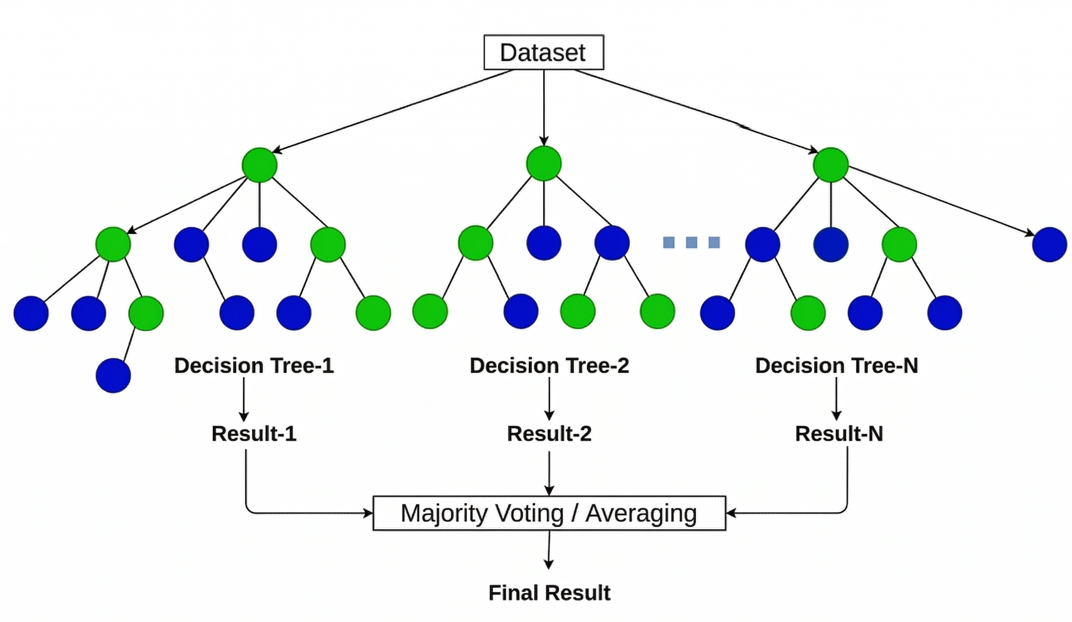 Figure 1: RF algorithm process (Source: Jain, A.)
2. Methodology: The 4-Step Process
Step 1: Bootstrap Sampling (Bagging)
Multiple training datasets are generated from the original data using bootstrap sampling (also called bagging, short for Bootstrap AGGregatING).
From the original training dataset of $n$ rows, $B$ bootstrap samples are generated. A bootstrap sample is drawn with replacement, meaning the same row can appear more than once, while some rows may not appear at all.
On average:
- Each bootstrap sample contains approximately 63% unique rows.
- The remaining 37%, called out-of-bag (OOB) samples, are left out of training for that tree. They serve as a built-in validation set, allowing the model to estimate its own error without needing a separate test set.
Each tree $b$ is trained on its own sample $\mathcal{D}^{*b}$:
\[\mathcal{D}^{*b} = \{ (\mathbf{x}_{i}^{*}, y_{i}^{*}) \}_{i=1}^{n} \sim \text{Sample with replacement from } \mathcal{D} \tag{1.1}\]Why does this help? Because each tree sees a slightly different version of the data, the trees make different errors. Averaging these uncorrelated errors reduces the overall variance of the model, without increasing its bias.
Step 2: Random Feature Selection
At each node split, the algorithm only considers a random subset of $m$ features out of $p$ total features. The best split is chosen from only those $m$ candidates, not from all features.
This step is what separates Random Forest from standard bagging. If all features were considered at every split, one dominant feature (such as temperature or wind speed) would appear at the root of nearly every tree. The trees would then be very similar to each other, and averaging them would give little benefit. By restricting the feature set at each split, the trees are decorrelated, which makes the ensemble much more powerful.
The default size of the feature subset is:
\[m = \begin{cases} \sqrt{p} & \text{for classification} \ p & \text{for regression} \end{cases} \tag{1.2}\]where $p$ is the total number of input features.
Step 3: Growing Decision Trees
Each tree is grown to its maximum depth without pruning. This intentionally allows individual trees to overfit their own bootstrap sample. A fully grown tree has low bias but high variance. This high variance is not a problem, because the aggregation step in Step 4 corrects it.
At each node, the algorithm selects the best split from the random subset of $m$ features using one of the following criteria:
For classification, the split minimizes the Gini Impurity (G):
\[G = 1 - \sum_{k=1}^{K} \hat{p}_{mk}^{2} \tag{1.3}\]Where $\hat{p}{mk}$ is the proportion of class $k$ samples at node $m$. A Gini value of 0 means a perfectly pure node, where all samples belong to the same class._
For regression, the split minimizes the Sum of Squared Errors (SSE):
\[\text{SSE} = \sum_{i \in \text{left}} (y_{i} - \bar{y}_{L})^{2} + \sum_{i \in \text{right}} (y_{i} - \bar{y}_{R})^{2} \tag{1.4}\]Where $\bar{y}{L}$ and $\bar{y}{R}$ are the mean target values of the left and right child nodes after the split. A smaller SSE means a better split.
Key insight: A single overfitted tree has high variance. It is very sensitive to small changes in the training data. However, when many such trees are averaged together in the next step, the variance decreases by roughly a factor of $1/B$, while the bias stays approximately the same.
Step 4: Aggregation
Once all $B$ trees are trained, their predictions are combined into a single final output. This step is what gives RF its stability.
For regression (Mean):
\[\hat{f}_{\text{RF}}(\mathbf{x}) = \frac{1}{B} \sum_{b=1}^{B} \hat{f}^{*b}(\mathbf{x}) \tag{1.5}\]Averaging reduces the variance by a factor of $1/B$ relative to a single tree, while the bias stays approximately unchanged.
For classification (Majority Vote):
\[\hat{y}_{\text{RF}}(\mathbf{x}) = \arg\max_{k} \sum_{b=1}^{B} \mathbb{1}(\hat{f}^{*b}(\mathbf{x}) = k) \tag{1.6}\]Where $k$ is the class label (for example, 0 or 1). The class that receives the most votes across all $B$ trees becomes the final prediction.
3. Hyperparameters
Tuning the hyperparameters of a Random Forest directly affects the balance between model accuracy and computational cost. The table below lists the key parameters and their effects.
| Parameter | Range | Effect |
|---|---|---|
n_estimators | 100 - 500 | Number of trees $B$. More trees improve stability but increase compute time. Test error plateaus and cannot rise by adding more trees, so there is no upper-bound overfitting risk. |
max_features | sqrt, log2 | Features considered per split $m$. Smaller values decorrelate trees more aggressively. Default: $m = \sqrt{p}$ for classification, $m = p$ for regression. |
max_depth | 10 - 30, None | Maximum depth of each tree. Deeper trees have lower bias but higher individual variance. None grows each tree fully, which is the standard RF setting before aggregation corrects the variance. |
min_samples_split | 2 - 20 | Minimum samples required to split a node. Higher values prevent splits on very small groups, reducing overfitting at the cost of slightly higher bias. |
min_samples_leaf | 5 - 20 | Minimum samples required at a leaf node. Prevents overly specific leaves, which is particularly important when the target variable contains many zero values. |
bootstrap | True | Whether to use bootstrap sampling. Disabling it removes the row randomness that decorrelates the trees and reverts to a standard ensemble on the full dataset. |
Tuning strategy: Parameters with a search range are tuned using an inner cross-validation loop. RMSE is minimised for regression; $F_{1}$ score is maximised for classification.
bootstrapandmax_featuresare fixed by design throughout.
4. Advantages and Limitations
Advantages
- Robustness: Highly resistant to outliers and noise. The ensemble structure means that no single noisy data point can dominate the final prediction.
- No overfitting risk from more trees: Unlike many models, adding more trees to a Random Forest does not cause overfitting. The test error plateaus but never increases.
- Feature Importance: RF naturally calculates which input variables contribute most to the predictions, using Gini impurity reduction. This is useful for understanding and interpreting the model.
- Works for both tasks: The same algorithm handles both regression and classification without major changes, which makes it easy to apply to different problems.
- Parallelization: Each tree is independent of the others, so all trees can be trained at the same time across multiple CPU cores.
Limitations
- Interpretability: A forest of hundreds of trees cannot be read or visualised as a simple set of rules. It is often called a “black box” model. Post-hoc tools like SHAP values are needed to explain individual predictions.
- Memory Usage: Deep forests with many trees can consume significant RAM, because memory scales linearly with the number of trees multiplied by the size of each tree. This should be monitored for large deployments.
- Slower prediction than a single tree: While training can be parallelised, making a prediction still requires passing input data through every tree in the forest, which is slower than a single decision tree.
5. Conclusion
Random Forest is a reliable and well-tested algorithm for both regression and classification tasks. Its design, built on bootstrap sampling and random feature selection, allows it to produce stable and accurate predictions even on noisy or imbalanced datasets. It requires relatively little tuning compared to other algorithms, and it provides native feature importance scores that help with model interpretation.
While it lacks the simple visual rules of a single tree, its stability and accuracy make it a strong choice for many real-world problems.
In the next post, we will present the practical application of Random Forest using Python.
References
- Breiman, L. (2001). Random Forests. Machine Learning, 45(1), 5-32. https://doi.org/10.1023/A:1010933404324
- Jain, A. Everything about Random Forest. Medium article