Fundamental of Electricity Markets (Part 1)
Published:
This post is the first in a series on the fundamentals of electricity markets in Europe. The contents are synthesized from two main lecture courses at Politecnico di Torino (PoliTo) and the KTH Royal Institute of Technology. Specific source documents are hyperlinked in the Sources section below.
- Part 1 (This post) covers:
- Fundamental economic and physical concepts in power systems (generation, transmission, distribution, utilization)
- Recall Math: Average vs. marginal costs
- Law of diminishing marginal utility and returns (demand and supply curves)
- Market equilibrium clearing and clearing price (MCP/MCQ)
- Surplus analysis: Consumer surplus, producer surplus, and social welfare
- Strategic bidding behavior of producers and market power
- Electricity as a unique commodity (non-storability, grid physics, reserves)
- The liberalization ladder (levels 0–3) and market participant roles
- Part 2 (Next post) will cover: (Note: Part 2 will be written when I finish my self-directed DTU course, which you can refer to here)
- Electricity market structures: pool model vs. bilateral model
- Day-Ahead Markets
- Intraday Markets
- Balancing Markets
- Ancillary Service Markets
- Impact of Renewable Energy on Electricity Markets
Electricity Markets
An electricity market is a system that enables the transfer of electric energy from producers to consumers, relying on a dedicated infrastructure - the power system.
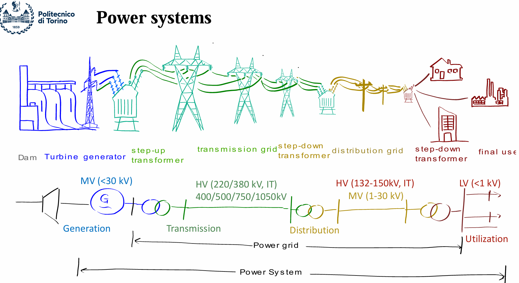
Fig 1: Power system
A power system is the physical network that generates electrical energy, transmits it over long distances, distributes it locally, and delivers it to consumers while maintaining stability, reliability, and quality. It includes:
- Generation: power plants (thermal, hydro, wind, solar, etc.) that produce electricity.
- Transmission: high‑voltage lines (HV, EHV) that move bulk power across long distances.
- Distribution: medium‑ and low‑voltage networks (MV, LV) that deliver electricity to cities, neighborhoods, and buildings.
- Utilization: all end‑user equipment that consumes electricity (homes, industries, commercial loads).
Recall Math - Average vs Marginal
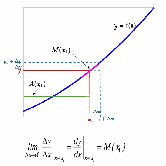
The function $f(x)$ gives the value of a quantity $y$ as a function of the variable $x$. For a specific point $x_1$ with corresponding value $y_1=f(x_1)$, we define:
$$A(x_1) = \frac{f(x_1)}{x_1}$$This represents the slope of the line connecting the origin to $(x_1, y_1)$.
For a small increase of the variable $x$, from $x_1$ to $x_1+\Delta x$, the quantity $y$ increases from $y_1$ to $y_1+\Delta y$. In the limit, the marginal value is defined as:
$$M(x_1) = \lim_{\Delta x \to 0} \frac{\Delta y}{\Delta x} = f'(x_1)$$This represents the slope of the function $f(x)$ at $x=x_1$.
Scarcity & Marginal Utility
| Concept | Scarcity | Law of Diminishing Marginal Utility |
|---|---|---|
| Definition | Resources are limited relative to demand. | Each additional unit consumed gives less added satisfaction (utility). |
| Core Idea | Not enough supply to satisfy all wants. | Utility gained from consuming extra units decreases. |
| Cause | Physical, economic, or technical limits (e.g., limited generation capacity). | Human behavior: satisfaction decreases as consumption increases. |
| Effect on Prices | Scarcity increases prices because demand > supply. | Consumers are willing to pay less for each additional unit. |
| Role in Markets | Drives competition and allocation of limited electricity. | Shapes demand curve and bidding behavior. |
| Example | Peak hours: limited generation → high prices. | First kWh is very valuable; the 100th kWh adds little extra benefit. |
Demand curves
• Utility always increases with the consumed quantity, but the utility of the last consumed unit decreases (marginal utility decreases). • The utility is reflected by the price the consumer is willing to pay. • Therefore, the demand curve represents the marginal utility of the good. • The demand curve $d(p)$ is a decreasing function, expressing the price buyers are willing to pay as a function of the quantity demanded: \(\nu = d(p)\) • The inverse demand curve expresses the quantity buyers demand as a function of the price: \(p = g(\nu)\)
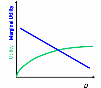
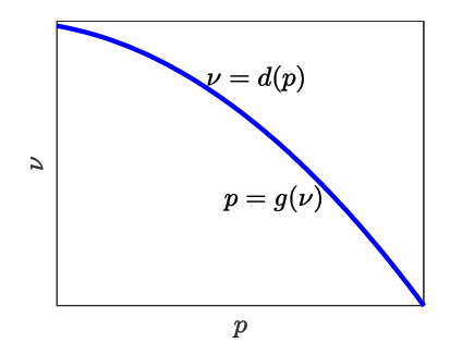
Fig 3 and 4: Demand curves
Costs
• Fixed cost $c_F$: cost that does not depend on the production quantity (land, machines, taxes…). • Variable cost $c_V(p)$: cost that depends on the production quantity (labor, fuel, electricity…). • Total cost $c(p)$: sum of fixed and variable costs: \(c(p) = c_F + c_V(p)\)
• Average cost: cost per unit at production level $p$: \(\bar{c}(p) = \frac{c(p)}{p}\)
• Average variable cost: \(\bar{c}_v(p) = \frac{c_V(p)}{p}\)
• Marginal cost $c_m(p)$: derivative of the total cost with respect to quantity: \(c_m(p) = \frac{dc(p)}{dp}\)
Law of diminishing marginal returns and supply curve
An increase in variable inputs relative to fixed inputs raises total output, but after a certain point the extra output from the same input increase becomes smaller.
- As production grows, producers must use increasingly costly resources.
- Since marginal cost rises with output, the supply curve is upward‑sloping.
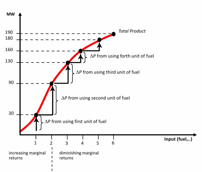
Fig 5: Diminishing marginal returns
Cost, Price, and Profit
• Cost: the total economic expenditure a firm must undertake to produce a given quantity of a good. It includes all resources used in production. • Price: the monetary value assigned to one unit of the good in the market; it reflects consumers’ willingness to pay and producers’ willingness to sell. • Profit: the financial gain obtained by a firm, equal to the difference between the revenue from selling the good and the total cost of producing it. A rational firm aims to maximize profit.
Equilibrium and Market Clearing Price
- Equilibrium: the condition in which the quantity offered by sellers equals the quantity demanded by buyers at a specific price.
- When price is higher than $\lambda$ ($v_2$), more quantity is produced but less quantity is demanded, prompting producers to decrease the price.
- When price is lower than $\lambda$ ($v_1$), more quantity is demanded but less quantity is produced, prompting buyers to increase their bids, raising the price.
- Market Clearing Price (MCP): the unique price at which supply and demand are exactly equal, ensuring that all offered quantity is sold and all demanded quantity (Market Clearing Quantity (MCQ)) is purchased.
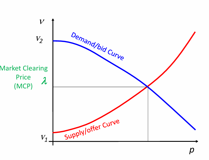
Fig 6: Equilibrium and Market Clearing Price
Consumer Surplus, Producer Surplus, and Social Surplus
| Concept | Definition |
|---|---|
| Consumer Surplus | The economic benefit consumers receive when they pay a market price lower than the maximum they were willing to pay. |
| Producer Surplus | The economic benefit producers receive when the market price is higher than the minimum price at which they were willing to supply the good. |
| Social Surplus | The total economic benefit created in the market, equal to the sum of consumer surplus and producer surplus. |
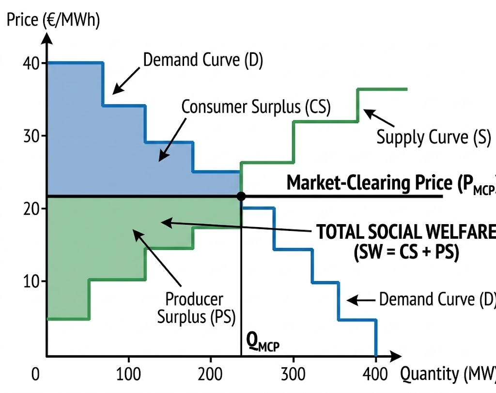
Fig 7: Consumer Surplus, Producer Surplus, and Social Surplus
Strategic Bidding Behavior of Producers
In a perfectly competitive market, producers offer electricity at their true marginal cost. This keeps the market‑clearing price low and ensures the market operates efficiently, maximizing social surplus. Consumers pay a fair price, producers earn normal profit, and the market clears at the socially optimal point where supply equals demand. In the diagram, this is shown on the left side: the demand curve intersects the marginal cost curve at the competitive equilibrium. The blue area represents consumer surplus, the orange area represents producer surplus, and together they form the total social surplus, which is maximized.
In a market where producers have market power, they can bid strategically by offering electricity at a higher price than their real cost. This pushes the market‑clearing price upward, increasing producer surplus but reducing consumer surplus and overall social welfare. For example, if a generator’s true marginal cost is €40/MWh but it submits an offer at €60/MWh, the market price may rise to €60/MWh instead of €40/MWh. Producers earn more, consumers pay more, and the market clears at a less efficient point that benefits producers at the expense of society.
In the diagram, this appears on the right side: the strategic offer curve lies above the marginal cost curve, leading to a higher price and lower quantity. The red triangle shows the deadweight loss - the lost social welfare caused by strategic bidding.
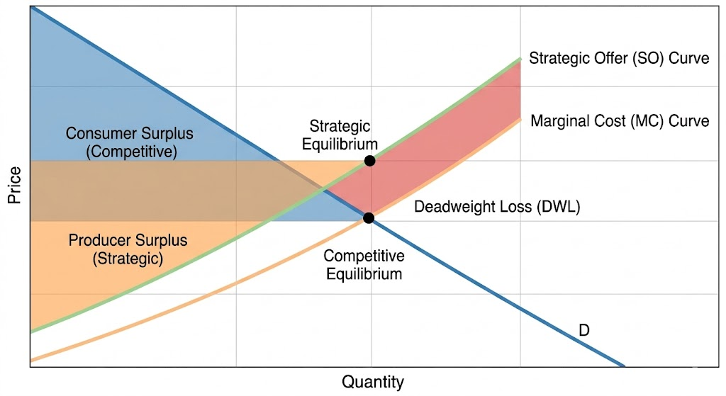
Fig 8: Demand diagram showing strategic bidding behavior of producers
Electricity as a commodity
Electricity is fungible, like gold, oil, or copper - one unit is interchangeable with another, and price is the only thing that tells two offers apart. But unlike those commodities, there are several factors making electricity different:
- No large-scale storage: Production has to equal consumption instantly, everywhere on the grid. Hydro reservoirs are about the only large-scale option, and even they lose energy round-trip (~74% efficiency). France, for example, has ~250 GW of subscribed consumption capacity vs only ~128 GW installed.
- Delivery quality matters: Power has to stay within tight bounds on frequency, voltage, and harmonics; reactive power is needed to deliver real power even though it does no useful work itself.
- Flows ≠ contracts: Where electricity actually goes is decided by the grid’s physics, not by who bought it from whom (e.g., Kirchhoff’s Laws).
- Consequence: An unresolved imbalance shows up as a frequency deviation, and left uncorrected, cascades into a blackout.
- TSO reserves exist to cover exactly this: primary (<20s, automatic), secondary (<3min), tertiary (<15min, manual).
From monopoly to competition: liberalization levels
- Level 0: Monopoly, fully bundled, regulated
- Level 1: Purchasing agency, competition only in generation
- Level 2: Wholesale competition, retailers/large customers choose supplier
- Level 3: Retail competition, everyone chooses supplier
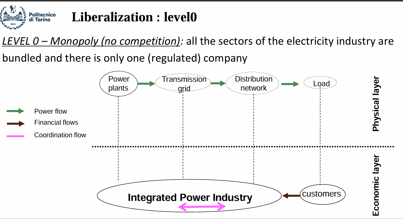
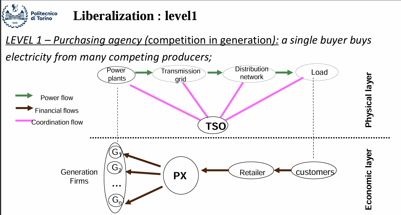
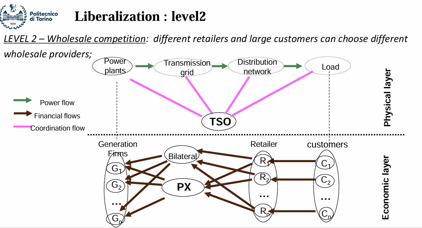
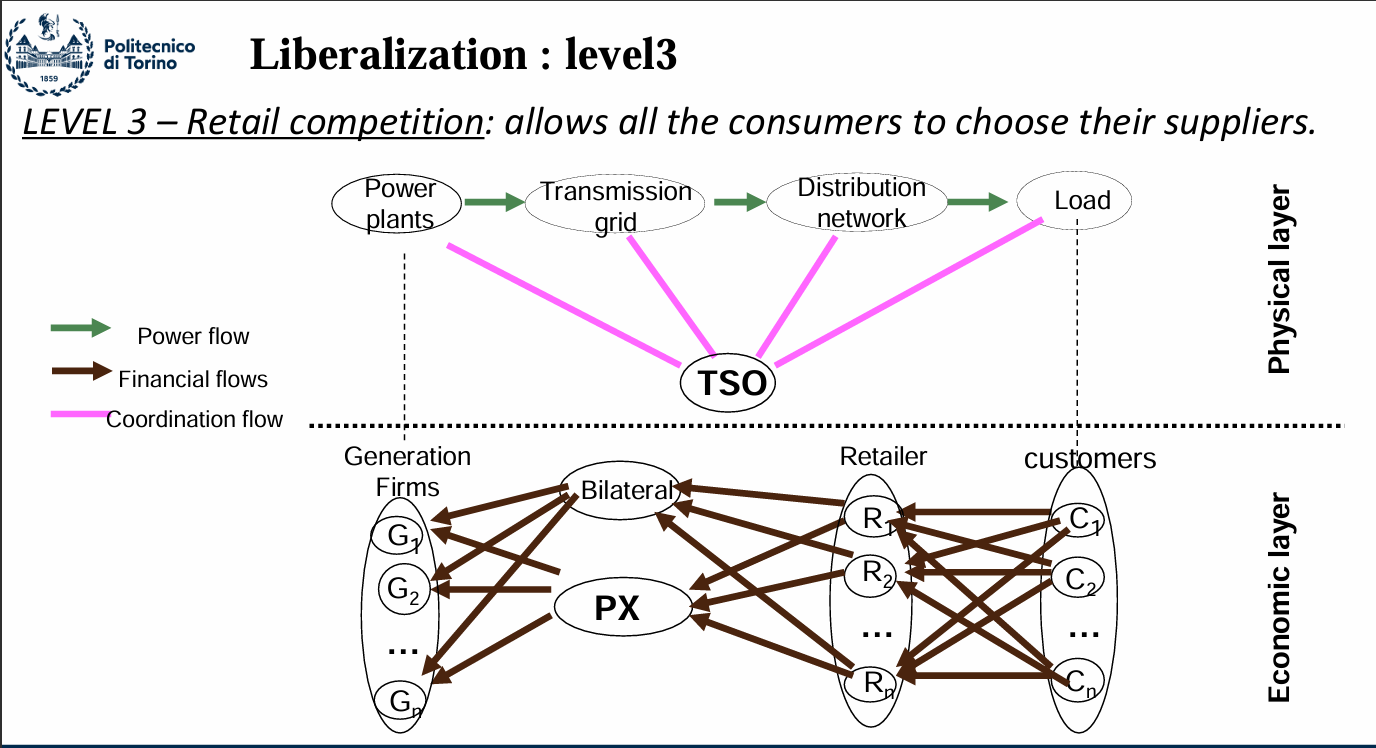
Fig 9 to 12: liberalization ladder 0–3
From regulation to liberalization
Electricity systems moved from one regulated monopoly controlling generation, transmission, distribution, and retail to a liberalized structure where generation and retail are opened to competition, while transmission and distribution remain regulated natural monopolies.
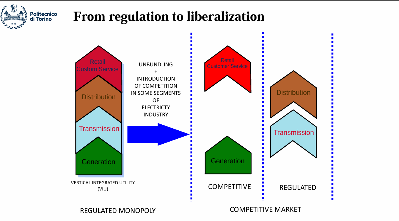
Fig 13: From regulation to liberalization
Functions in Electricity Market
- Producers: Generate electricity and submit offers to the market. They decide how much to produce and at what price, aiming to maximize profit.
- Power Demands & Consumers:
- Large Consumers: Large-scale users (e.g., industrial plants, factories) who consume significant volumes of electricity and often participate directly in the wholesale market.
- Retailers: Intermediate market actors (or traders) who purchase electricity in bulk from the wholesale market and resell it to smaller end-consumers (e.g., households, commercial buildings) who do not have direct market access.
- Market Operator: A non-profit entity that receives all offers from producers and bids from consumers, clears the market by maximizing social welfare, and distributes the final market-clearing outcomes (prices and quantities).
- System Operators & Grid Owners:
- Transmission System Operator (TSO): Responsible for the safe and reliable operation of the high-voltage transmission grid (typically a meshed network with many loops). They ensure supply security, real-time power balance, and system stability.
- Note: In Europe, ENTSO-E (European Network of Transmission System Operators for Electricity) represents all European TSOs working together to run the grid and coordinate cross-border markets.
- Distribution System Operator (DSO): Responsible for the safe and reliable operation of the medium- and low-voltage distribution networks (typically radial grids, which are tree-like structures where electricity flows in one direction from substations to consumers with no loops).
- Transmission System Operator (TSO): Responsible for the safe and reliable operation of the high-voltage transmission grid (typically a meshed network with many loops). They ensure supply security, real-time power balance, and system stability.
- Market Regulator: Responsible for monitoring market performance in both the short and long run, ensuring fair competition, and designing appropriate market regulations and policies.
- Traders: Participate in buying and selling electricity across different timeframes and markets to profit from price differences. They can engage in both physical trading (requiring actual delivery) and purely financial trading.
- Balance Responsible Parties (BRPs): Market participants (or entities representing them) that are financially responsible for keeping their portfolio’s production and consumption schedules balanced. Any real-time deviations from their schedules incur imbalance costs.
- Flexibility Aggregators: Service providers who group multiple smaller distributed energy resources (such as electric vehicles, smart appliances, or batteries) to offer flexibility and balancing services to TSOs and DSOs.
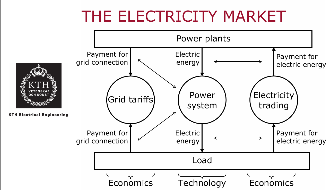
Fig 14: Functions in Electricity Market
Sources
- KTH Royal Institute of Technology: Course “EG2050 System Planning”, taught by Prof. Mikael Amelin.
- Lecture 1 - 2: The Structure of an electricity market (2014) — Download Lecture Slides (PDF)
- Politecnico di Torino (PoliTo): Course “Smart Electricity Systems”, taught by Prof. Tao HUANG.
- Lecture 1: A Crash Introduction to (Smart) Power Systems — Download Lecture Slides (PDF)
- Lecture 2: Markets for electricity (A.Y. 2025-2026) — Download Lecture Slides (PDF)
- AI Artworks: Figures 7 and 8 generated using Gemini AI.