Smart Heat Pump Control: Reinforcement Learning and Digital Twins
Published:
1. Goal
The objective of this project is to develop an intelligent controller for a residential heat pump coupled with a thermal energy storage (TES) tank. The goal is to minimize total electricity costs by shifting electricity demand to lower-priced hours (arbitrage) while satisfying the building’s heat demand and maintaining the storage water temperature within physical and operational safety boundaries.
2. Methodology
The pipeline integrates a physics-based model of the thermal storage tank with a machine learning corrector (the Digital Twin) and a Reinforcement Learning (RL) control agent.
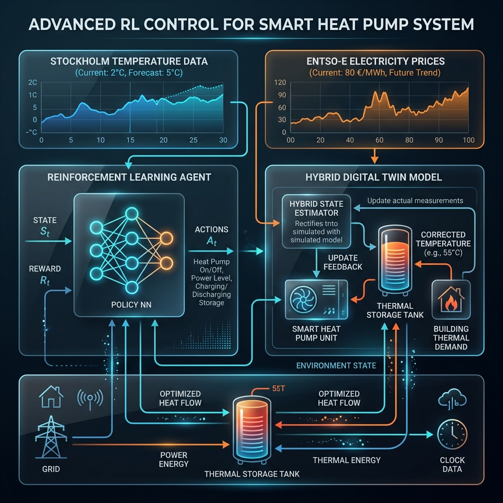
- Data Ingestion and Alignment: Import local hourly outdoor temperature data and day-ahead electricity prices.
- Environment Modeling: Build a custom Gymnasium environment representing the physical heat pump and storage tank.
- Digital Twin Development: Train a Gradient Boosting Regressor on simulated residual data to correct discrepancies between the simplified physics model and actual system behavior.
- RL Agent Training: Train a Proximal Policy Optimization (PPO) agent to learn optimal control policies over a continuous action space.
- Performance Evaluation: Analyze cost savings and constraint satisfaction over a one-week deterministic rollout.
3. Input Data
3.1 ERA5 Temperature Data
Outdoor temperature data is sourced from the ERA5 hourly reanalysis dataset on pressure levels (950 hPa) for the Stockholm zone using the following bounding box:
- North: $59.50^\circ$
- South: $59.10^\circ$
- West: $17.80^\circ$
- East: $18.30^\circ$
Temperature values are converted from Kelvin to Celsius and spatially averaged across the grid coordinates.
3.2 Day-Ahead Electricity Prices
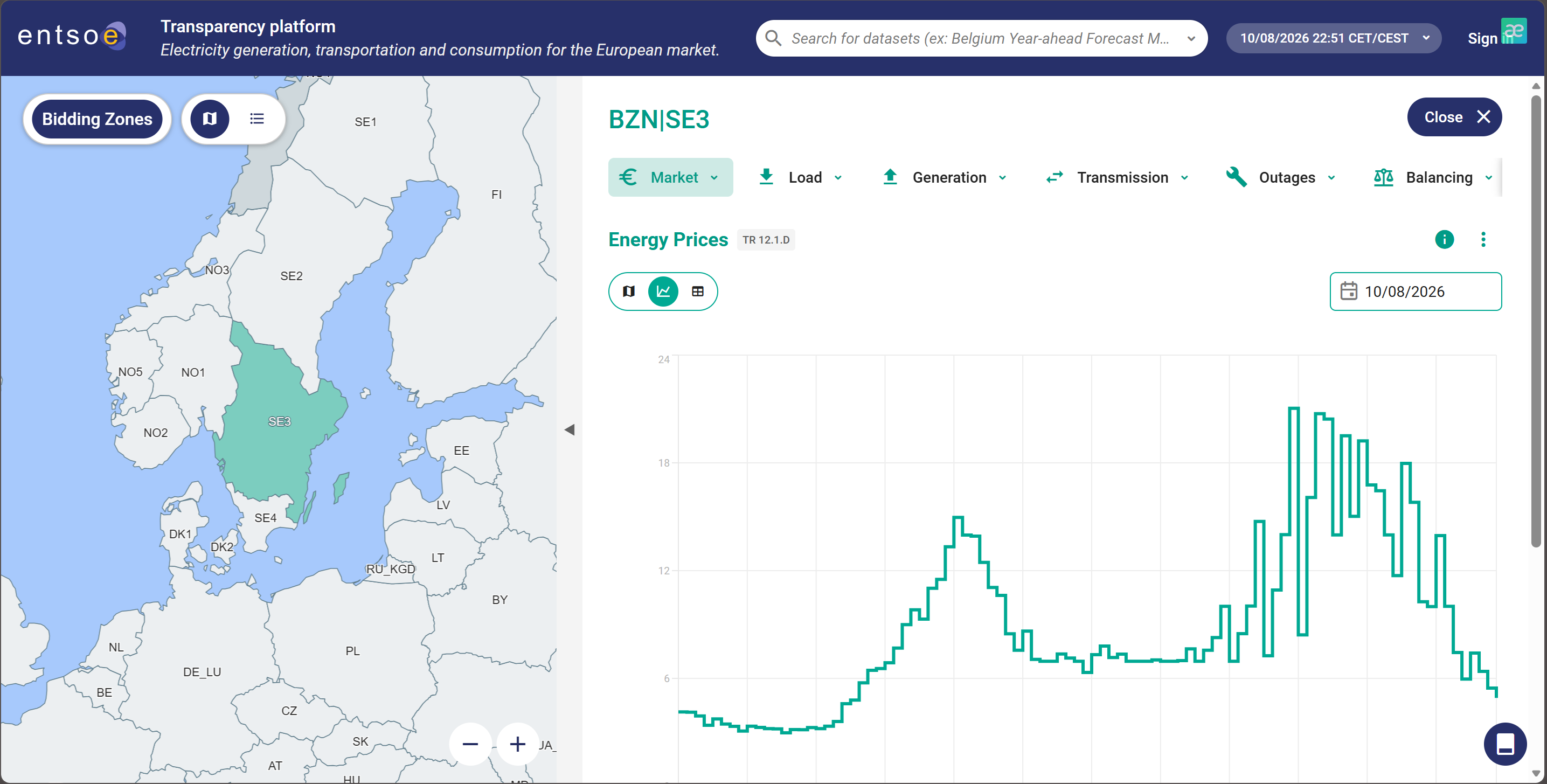
Historical day-ahead spot prices for the SE3 region (Stockholm) are sourced from the ENTSO-E Transparency Platform (available at transparency.entsoe.eu). The spot prices are published daily, giving the agent a complete, noise-free 24-hour lookahead window.
4. Heat Pump & Storage Tank Assumptions
| Parameter | Symbol | Value | Unit | Description |
|---|---|---|---|---|
| Max Electrical Power | $P_{\text{max}}$ | $10.0$ | $\text{kW}$ | Max electrical input to the compressor. |
| Thermal Capacity | $C$ | $50.0$ | $\text{kWh/K}$ | Storage tank thermal mass (equivalent to $\sim 860$ L of water). |
| Tank Loss Coefficient | $\beta$ | $0.03$ | $\text{kW/K}$ | Heat loss rate from storage tank to ambient air, for a well-insulated tank. |
| Building Load Coefficient | $k_h$ | $0.3$ | $\text{kW/K}$ | Building heat demand coefficient relative to an $18^\circ\text{C}$ indoor baseline. |
| Minimum Temperature | $T_{\text{min}}$ | $40.0$ | $^\circ\text{C}$ | Lower operational limit of the storage tank ($\text{SOC} = 0$). |
| Maximum Temperature | $T_{\text{max}}$ | $80.0$ | $^\circ\text{C}$ | Upper operational limit of the storage tank ($\text{SOC} = 1$). |
COP Model: The Coefficient of Performance varies linearly with ambient temperature:
\[\text{COP}(T_{\text{amb}}) = \text{COP}_0 + \alpha \cdot (T_{\text{amb}} - 5)\]where $\text{COP}_0 = 3.0$ and temperature sensitivity coefficient $\alpha = 0.05$.
These values were chosen so that the heat pump has spare thermal capacity year-round: even at the coldest hour in the dataset ($-12^\circ\text{C}$), maximum compressor output still exceeds building demand plus tank losses by a wide margin. That headroom is what makes load-shifting possible at all. With a tighter energy balance, the agent would have to run near-constantly just to keep the tank from draining, regardless of price.
5. Reinforcement Learning & Digital Twin Formulation
5.1 Markov Decision Process (MDP)
- State Space: \(s_t = \left[ T_{\text{amb}}(t), \text{SOC}(t), \text{Price}(t), \sin(\text{hour}), \cos(\text{hour}), \text{Price}_{t+1}, \dots, \text{Price}_{t+24} \right]\)
- Action Space: Continuous action $a_t \in [0, 1]$, representing the electricity input fraction of the heat pump compressor: $P_{\text{elec}} = a_t \cdot P_{\text{max}}$.
Reward Function: Minimizes operational cost and penalizes exceeding safety limits ($SOC \notin [0.05, 0.95]$):
\[R_t = - \Big( \text{Price}(t) \cdot P_{\text{elec}}(t) \cdot dt \Big) - w_{\text{penalty}} \cdot \max\Big(0, 0.05 - \text{SOC}_t, \text{SOC}_t - 0.95\Big)^2\]
5.2 Digital Twin State Correction
The simplified physical model estimates the temperature using:
\[T_{\text{physics}}(t+1) = T_{\text{physics}}(t) + \frac{(Q_{\text{hp}} - Q_{\text{heat}} - Q_{\text{loss}}) \cdot dt}{C}\]To emulate unmodeled effects such as pipe degradation or insulation leaks, a Gradient Boosting model is trained on residuals between a “true” environment and a deliberately drifted one ($C=42$ kWh/K, $\beta=0.036$ kW/K, roughly 15-20% off the true parameters). It predicts the mismatch between the true and physics-model state of charge, from the state $[T_{\text{amb}}, \text{SOC}, \text{Price}]$:
\[\Delta \text{SOC} = \text{SOC}_{\text{true}} - \text{SOC}_{\text{physics}}\]and the RL agent is always fed the corrected state:
\[\text{SOC}_{\text{corrected}} = \text{SOC}_{\text{physics}} + \Delta \text{SOC}\]5.3 Training Configuration
The corrector is a GradientBoostingRegressor (n_estimators=100, max_depth=5, random_state=42) trained on 17,520 simulated transitions.
The control policy is trained with Proximal Policy Optimization (Stable-Baselines3):
| Hyperparameter | Value |
|---|---|
| Policy network | MlpPolicy |
| Learning rate | 3e-4 |
Steps per update (n_steps) | 2048 |
| Batch size | 64 |
Epochs per update (n_epochs) | 10 |
| Discount factor ($\gamma$) | 0.99 |
| Entropy coefficient | 0.01 |
| Total training timesteps | 150,000 |
| Device | CPU |
The environment’s reward mixes two very different scales: a per-step electricity cost of a few cents against a safety penalty that can spike into the hundreds. Fed raw into PPO, that imbalance stalls the value function entirely, and the policy collapses onto a single “safe” constant action instead of learning a control strategy. Wrapping training in Stable-Baselines3’s VecNormalize (norm_obs=True, norm_reward=True, clip_reward=10.0) keeps a running estimate of reward scale and normalizes both observations and rewards before they reach the network. Without that normalization, the reward signal is not learnable. The same running statistics are reused at evaluation time to normalize observations before inference, so the policy always sees inputs on the scale it was trained on.
Dependencies: numpy, pandas, xarray, gymnasium, scikit-learn, joblib, stable-baselines3, matplotlib (see requirements.txt in the Code section below for pinned versions).
6. Results & Discussion
Evaluated deterministically over one week (168 hours) starting February 11:
| Metric | Value |
|---|---|
| Total electricity consumed | 365.05 kWh |
| Total operating cost | EUR 14.03 |
| Average price paid | EUR 38.42/MWh |
| Average market price | EUR 52.32/MWh |
| Cost reduction vs. market average | 26.6% |
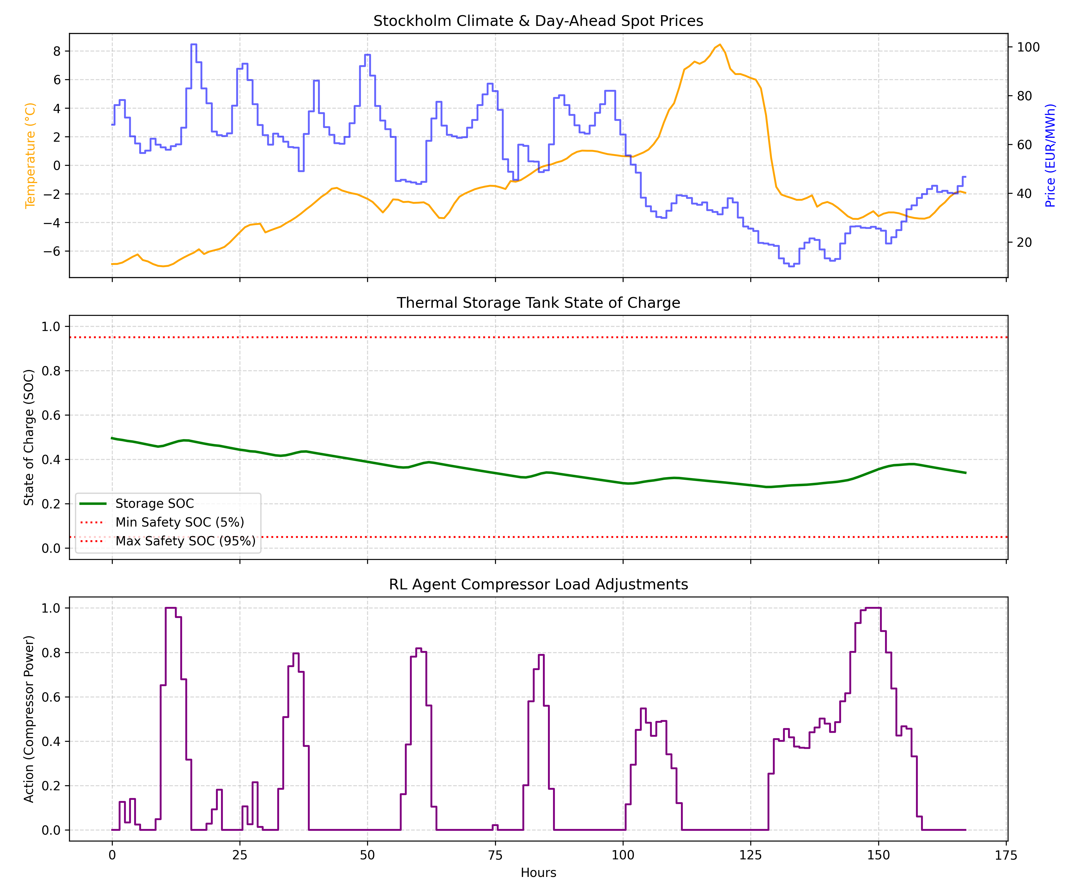
- Arbitrage behavior: compressor action and electricity price are negatively correlated (Pearson $r = -0.45$) over the evaluation week. The agent runs the heat pump harder when prices are low and eases off when they spike, using the tank as a buffer rather than a fixed-setpoint thermostat.
- Constraint satisfaction: storage SOC stays within $[0.275, 0.495]$ throughout the week, comfortably inside the $[0.05, 0.95]$ safety band. Feeding the agent the digital-twin-corrected state, rather than the raw physics estimate, keeps it from misjudging how much thermal buffer it actually has.
- Why the reward scale mattered: earlier runs of this same setup, evaluated without reward normalization, converged to a policy that never activated the compressor at all. That is a locally rational response to a reward signal dominated by rare, huge penalty spikes rather than the everyday cost trade-off. Normalizing the reward before training is what surfaces the price-arbitrage incentive to the optimizer.
Code
- environment/heatpump_env.py: the custom Gymnasium environment, covering tank thermal dynamics, the COP model, and the digital-twin correction hook.
- pipeline.py: the full pipeline (data processing, digital-twin training, PPO training, evaluation) as one script with
--stage {data,corrector,train,evaluate,all}. - requirements.txt: pinned package versions used to produce the results above.
Results/folder: evaluation_results.csv and evaluation_summary.txt.